Opticks : GPU Optical Photon Simulation for Particle Physics with NVIDIA OptiX
Opticks : GPU Optical Photon Simulation for Particle Physics with NVIDIA® OptiX™
Simon C Blyth, IHEP, CAS — https://bitbucket.org/simoncblyth/opticks — July 2018, CHEP, Sofia
Opticks Benefits
Outline
- Problem and approach to solving
- optical photon simulation problem
- GPU ray tracing solution
- NVIDIA OptiX ray tracing engine
- G4 Geometry translation to GPU
- general CSG boolean intersection
- auto-translated without approximation
- simplified direct workflow
- G4 Optical physics translation to GPU
- Hybrid Geant4/Opticks event workflow
- Validation with random sequence aligned running
- perfect match for simple geometries
- reveals CSG issues with full geometries
- Summary
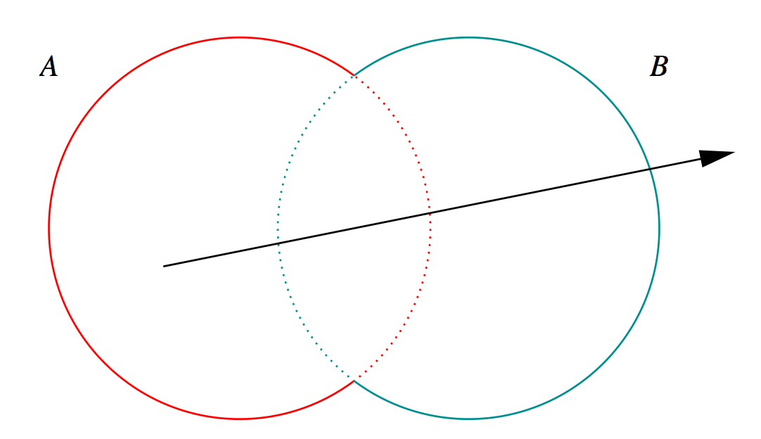
CSG : Constructive Solid Geometry, using boolean tree representation
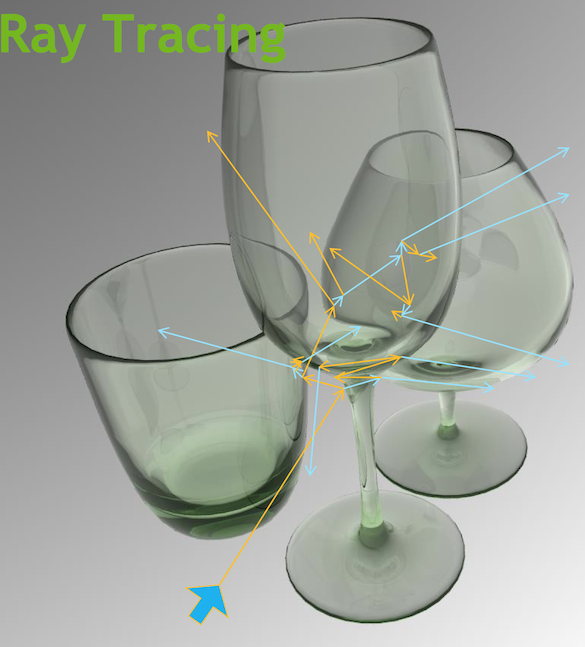
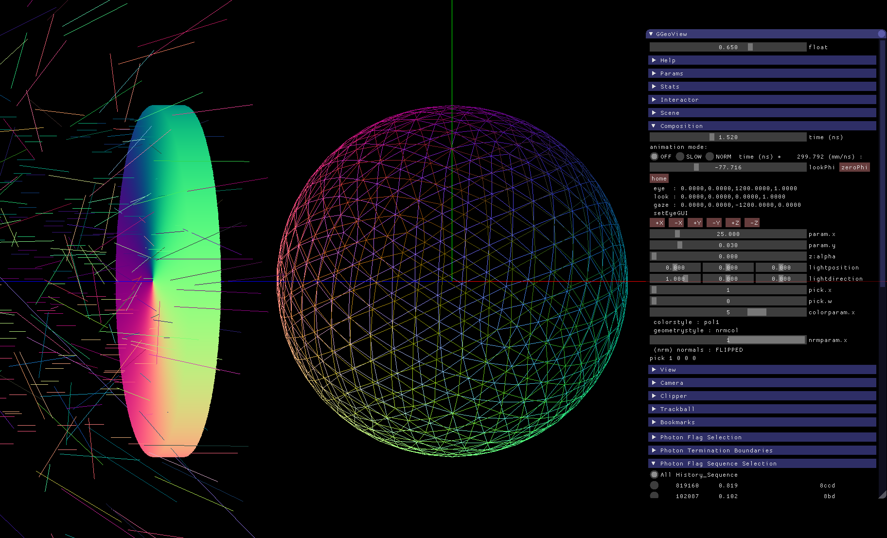
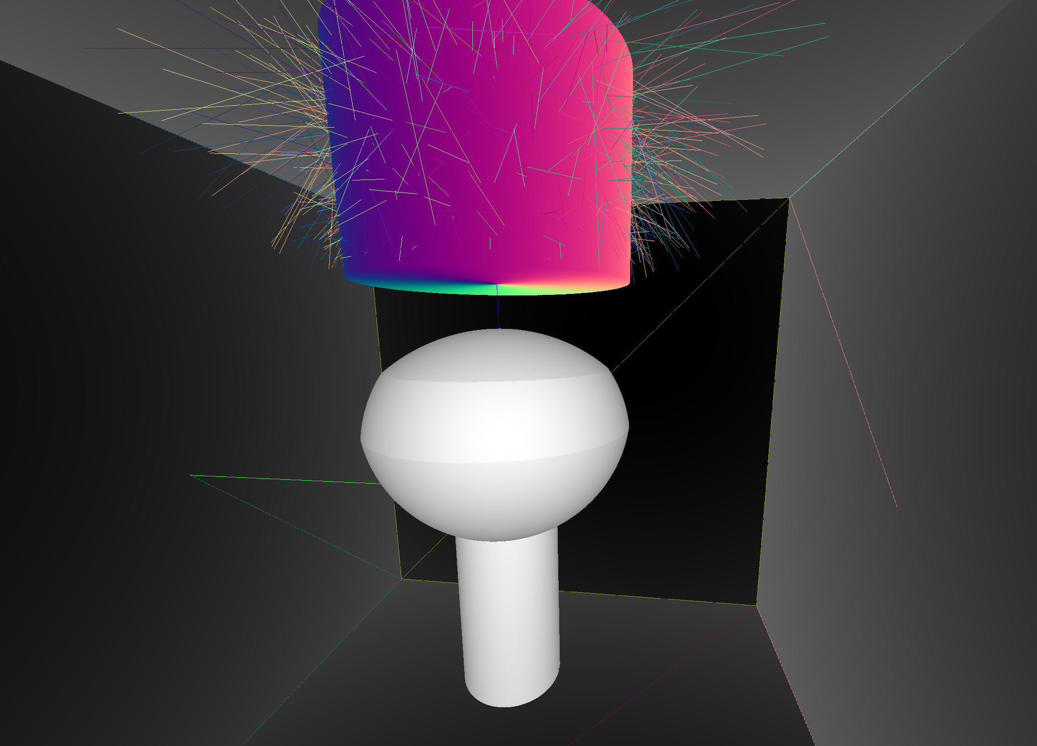
Optical Photon Simulation Problem...
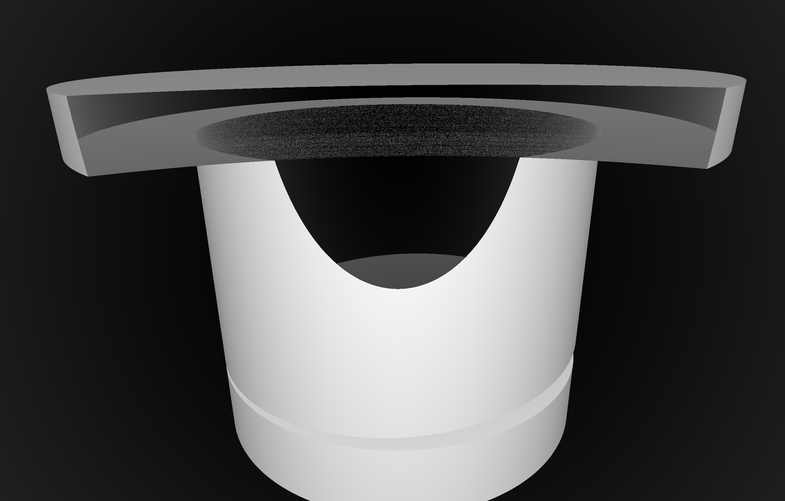
JPMT Before Contact 2
Ray Traced Image Synthesis ≈ Optical Photon Simulation
Geometry, light sources, optical physics ->
- pixel values at image plane
- photon parameters at detectors (eg PMTs)
Ray tracing has many applications :
- advertising, design, entertainment, games,...
- BUT : most ray tracers just render images
Ray-geometry intersection
- hw+sw continuously optimized over 30 years
- performance > 100M intersections per second per GPU
- rasterization
- project 3D primitives onto 2D image plane, combine fragments into pixel values
- ray tracing
- cast rays thru image pixels into scene, recursively reflect/refract at
intersects, combine returns into pixel values
Opticks : GPU Geometry starts from ray-primitive intersection
- 3D parametric ray : ray(x,y,z;t) = rayOrigin + t * rayDirection
- implicit equation of primitive : f(x,y,z) = 0
- -> polynomial in t , roots: t > t_min -> intersection positions + surface normals
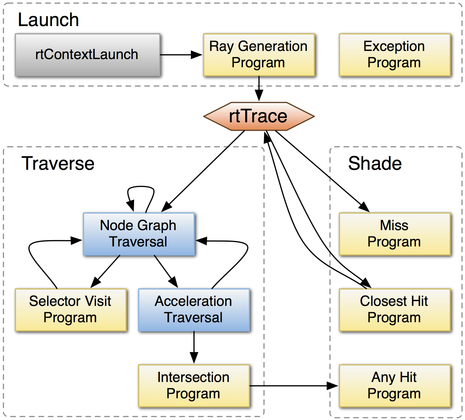
Ray intersection with general CSG binary trees, on GPU
Pick between pairs of nearest intersects, eg:
| UNION tA < tB |
Enter B |
Exit B |
Miss B |
|---|
| Enter A |
ReturnA |
LoopA |
ReturnA |
| Exit A |
ReturnA |
ReturnB |
ReturnA |
| Miss A |
ReturnB |
ReturnB |
ReturnMiss |
- Nearest hit intersect algorithm [1] avoids state
- sometimes Loop : advance t_min , re-intersect both
- classification shows if inside/outside
- Evaluative [2] implementation emulates recursion:
- recursion not allowed in OptiX intersect programs
- bit twiddle traversal of complete binary tree
- stacks of postorder slices and intersects
- Identical geometry to Geant4
- solving the same polynomials
- near perfect intersection match
- [1] Ray Tracing CSG Objects Using Single Hit Intersections, Andrew Kensler (2006)
- with corrections by author of XRT Raytracer http://xrt.wikidot.com/doc:csg
- [2] https://bitbucket.org/simoncblyth/opticks/src/tip/optixrap/cu/csg_intersect_boolean.h
- Similar to binary expression tree evaluation using postorder traverse.
CSG Complete Binary Tree Serialization -> simplifies GPU side
Geant4 solid -> CSG binary tree (leaf primitives, non-leaf operators, 4x4 transforms on any node)
Serialize to complete binary tree buffer:
- no need to deserialize, no child/parent pointers
- bit twiddling navigation avoids recursion
- simple approach profits from small size of binary trees
- BUT: very inefficient when unbalanced
Height 3 complete binary tree with level order indices:
                                                   depth     elevation

                     1                               0           3

          10                   11                    1           2

     100       101        110        111             2           1

 1000 1001  1010 1011  1100 1101  1110  1111         3           0
postorder_next(i,elevation) = i & 1 ? i >> 1 : (i << elevation) + (1 << elevation) ; // from pattern of bits
Postorder tree traverse visits all nodes, starting from leftmost, such that children
are visited prior to their parents.
Opticks Analytic Daya Bay Near Site, GPU Raytrace (3)
GPU raytrace : purely analytic geometry (Daya Bay Near Site)
Opticks Analytic Daya Bay Near Site, GPU Raytrace (1)
Opticks Analytic Daya Bay Near Site, GPU Raytrace (2)
Cutaway view of Daya Bay Antineutrino-detector
Opticks Analytic JUNO Chimney, GPU Raytrace (0)
JUNO Chimney at top of Central Detector Scintillator
Opticks : translates G4 geometry to GPU, without approximation
- Direct Geometry : Geant4 "World" -> Opticks CSG -> GPU
- simpler : no G4DAE+GDML export/import
- Material/Surface/Scintillator properties
- interpolated to standard wavelength domain
- interleaved into "boundary" texture
- "reemission" texture for wavelength generation
- Structure
- repeated geometry instances identified (progeny digests)
- instance transforms used in OptiX/OpenGL geometry
- merge CSG trees into global + instance buffers
- export meshes to glTF 2.0 for 3D visualization
- Ease of Use
- easy geometry : just handover "World"
- easy config : modern CMake + BCM[1]
- ~easy event : modify G4Cerenkov + G4Scintillation
[1] Boost CMake 3.5+ modules : configure direct dependencies only
https://github.com/BoostCMake/cmake_modules
https://github.com/simoncblyth/bcm
Opticks Export of G4 geometry to glTF 2.0
Opticks : translates G4 optical physics to GPU
OptiX : single-ray programming model -> line-by-line translation
- CUDA Ports of Geant4 classes
- G4Cerenkov (only generation loop)
- G4Scintillation (only generation loop)
- G4OpAbsorption
- G4OpRayleigh
- G4OpBoundaryProcess (only a few surface types)
- Modify Cerenkov + Scintillation Processes
- collect genstep, copy to GPU for generation
- avoids copying millions of photons to GPU
- Scintillator Reemission
- fraction of bulk absorbed "reborn" within same thread
- wavelength generated by reemission texture lookup
- Opticks (OptiX/Thrust GPU interoperation)
- OptiX : upload gensteps
- Thrust : seeding, distribute genstep indices to photons
- OptiX : launch photon generation and propagation
- Thrust : pullback photons that hit PMTs
- Thrust : index photon step sequences (optional)
Validation : Aligning CPU and GPU Simulations
Aligned zipping together of code and RNG values
- common input photon sample generated on CPU
- random number sequences generated on GPU (cuRAND)
and persisted to file (NPY buffers)
Single executable lldb OKG4Test:
- run Opticks GPU simulation, persist event
- run Geant4 simulation
- step-by-step check each G4 photon follows Opticks
history and parameters, break at deviations
- fix cause of misaligned RNG consumption, or other deviation
- tricks needed on both sides : burning RNGs, jump backs
simplest possible direct comparison validation
http://bitbucket.com/simoncblyth/opticks/src/tip/tools/autobreakpoint.py
(lldb) help breakpoint command add
Validation : Direct comparison of GPU/CPU NumPy arrays
tboolean-box simple geometry test
- 100k photons : position, time, polarization : 1.2M floats
- 34 deviations > 1e-4 (mm or ns), largest 4e-4
- deviants all involve scattering (more flops?)
In [11]: pdv = np.where(dv > 0.0001)[0]
In [12]: ab.dumpline(pdv)
      0   1230 : TO BR SC BT BR BT SA
      1   2413 : TO BT BT SC BT BR BR BT SA
      2   9041 : TO BT SC BR BR BR BR BT SA
      3  14510 : TO SC BT BR BR BT SA
      4  14747 : TO BT SC BR BR BR BR BR BR BR
      5  14747 : TO BT SC BR BR BR BR BR BR BR
    ...

In [20]: ab.b.ox[pdv,0]                                 In [21]: ab.a.ox[pdv,0]
Out[20]:                                                Out[21]:
A()sliced                                               A()sliced
A([    [-191.6262, -240.3634,  450.    ,    5.566 ],    A([    [-191.626 , -240.3634,  450.    ,    5.566 ],
       [ 185.7708, -133.8457,  450.    ,    7.3141],           [ 185.7708, -133.8456,  450.    ,    7.3141],
       [-450.    , -104.4142,  311.143 ,    9.0581],           [-450.    , -104.4142,  311.1431,    9.0581],
       [  83.6955,  208.9171, -450.    ,    5.6188],           [  83.6954,  208.9172, -450.    ,    5.6188],
       [  32.8972,  150.    ,   24.9922,    7.6757],           [  32.8973,  150.    ,   24.992 ,    7.6757],
       [  32.8972,  150.    ,   24.9922,    7.6757],           [  32.8973,  150.    ,   24.992 ,    7.6757],
       [ 450.    , -186.7449,  310.6051,    5.0707],           [ 450.    , -186.7451,  310.605 ,    5.0707],
       [ 299.2227,  318.1443, -450.    ,    4.8717],           [ 299.2229,  318.144 , -450.    ,    4.8717],
 ...
http://bitbucket.com/simoncblyth/opticks/src/tip/notes/issues/tboolean_box_perfect_alignment_small_deviations.rst
Coincident Faces are Primary Cause of Issues : Fake Intersects
Coincidences common (alignment too tempting?). To fix:
- A-B : grow correct dimension of subtracted shape
- A+B : grow smaller interface shape into bigger, making join
- case-by-case fixes straightforward, not so easy to automate
- WIP: automated coincidence finder/fixer
Opticks Users Group
List of "backup" slides
CSG
- Constructive Solid Geometry (CSG) : Shapes defined "by construction"
- CSG : Which primitive intersect to pick
- Ray Tracing CSG Objects Using Single Hit Intersections (A. Kensler)
- CSG Complete Binary Tree Serialization -> simplifies GPU side
- Evaluative CSG intersection Pseudocode : recursion emulated
- Opticks CSG Primitives : Closed Solids, Consistent Normals
- Opticks CSG Primitives : What is included
- Opticks CSG : Balancing Deep Trees Drastically Improves Performance
- Dayabay ESR reflector : Deep CSG tree : disc with 9 holes
- Opticks CSG Serialized into OpticksCSG format (numpy buffers, json)
Validation
- tconcentric : spherical GdLS/LS/MineralOil
- tconcentric : Opticks/Geant4 chi2 comparison
- tconcentric : Opticks/Geant4 distrib chi2/df ~ 1.0
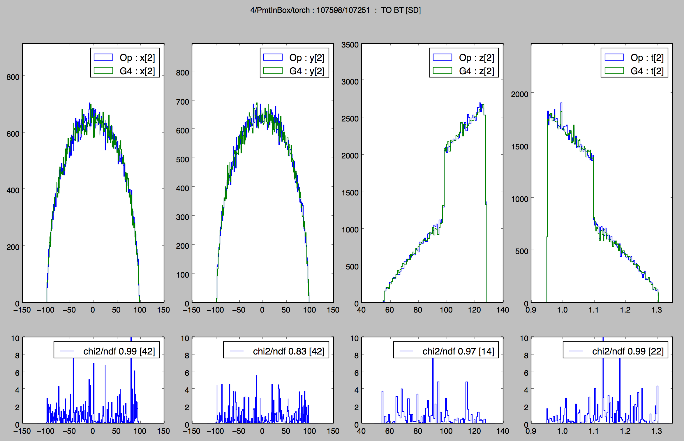
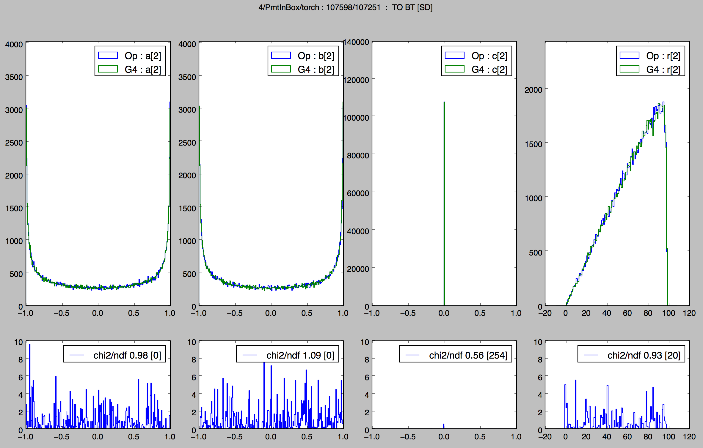
- PMT Opticks/Geant4 step distribution comparison TO BT [SD]
- PMT Opticks/Geant4 step distribution comparison : chi2/ndf
- Opticks/Geant4 Rainbow Step Sequence Comparison
- 1M Rainbow S-Polarized, Comparison Opticks/Geant4
- Compare Opticks/Geant4 Simulations with Simple Lights/Geometries
Misc
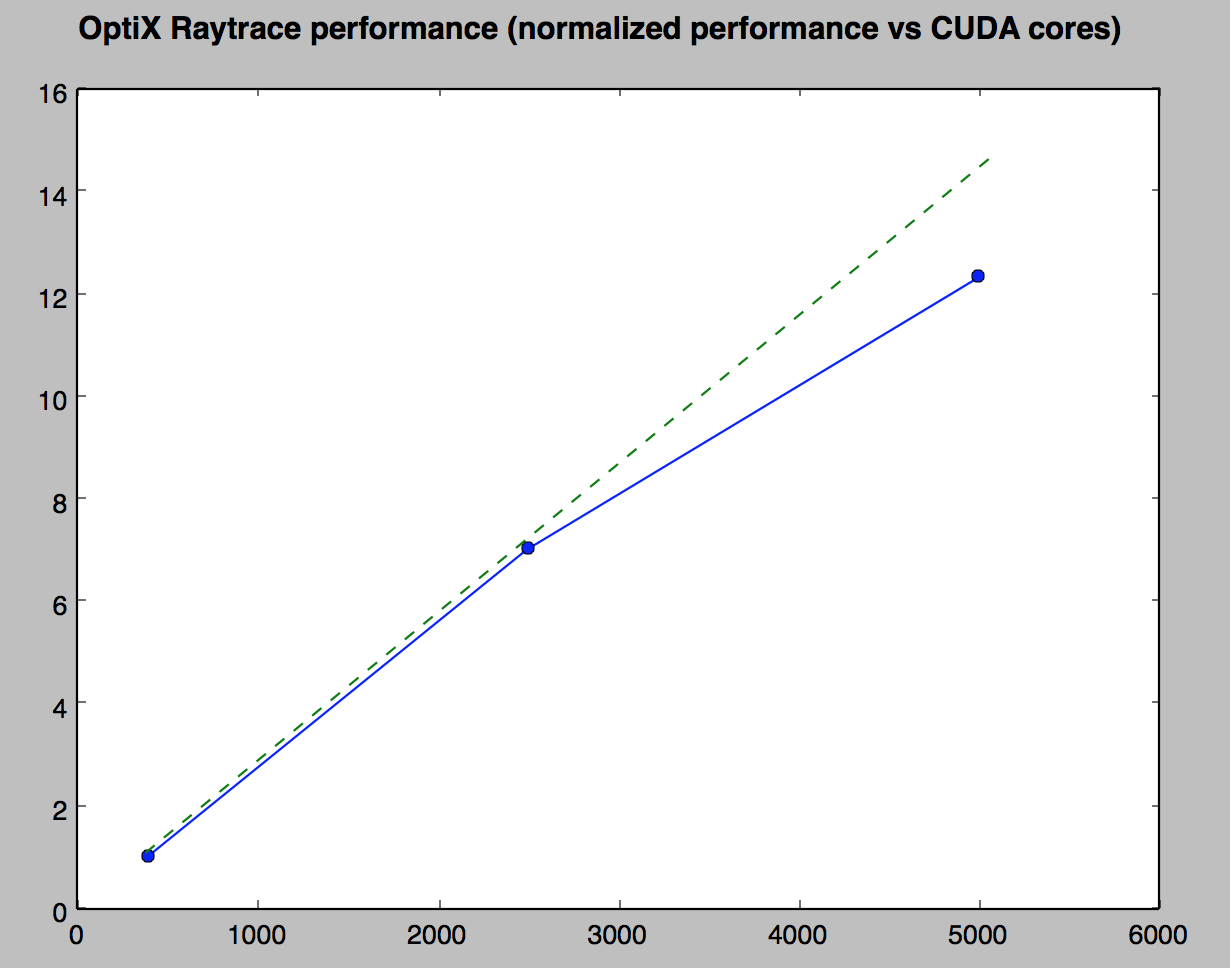
- OptiX Performance Scaling with GPU cores
- Torus : much more difficult/expensive than other primitives
- Geometry Modelling : Tesselated vs Analytic Photomultiplier Tubes
- Hybrid Geant4/Opticks Event Workflow
- Open Source Opticks
Idealized geometry tests : photon generation, propagation, reemission
Idealized "tconcentric" scintillator detector avoids any geometry issues, tests optical physics in isolation
Single executable (cfg4 package):
- performs both pure G4 and hybrid G4+Opticks simulations
- writes two events recording up to 16 steps of each photon
- photons indexed on GPU by history and material sequences
- history category counts comparison, Opticks/G4 chi2/df ~ 1.0
- position, time, polarization, wavelength recorded at each step
point-by-point chi2-distance comparisons of 8 photon properties for top 100 history categories
NEXT STEPS
- JUNO integration + full JUNO geometry validation
https://bugzilla-geant4.kek.jp/show_bug.cgi?id=1275
Photon Propagation Times Geant4 cf Opticks
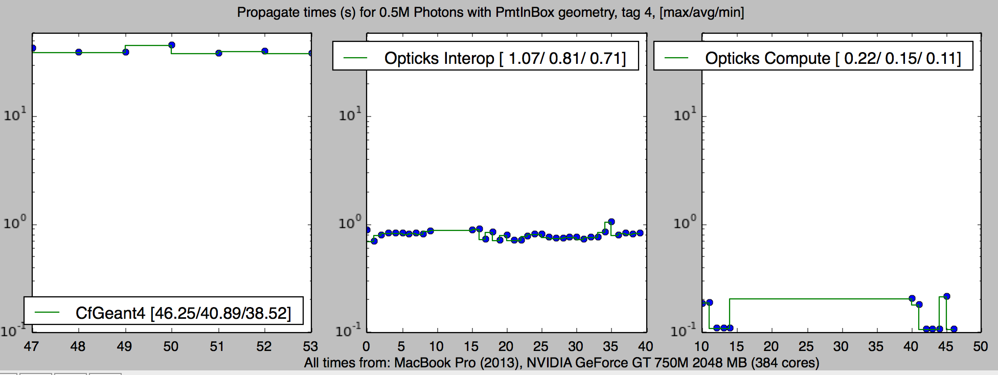
| Test |
Geant4 10.2 |
Opticks Interop |
Opticks Compute |
|---|
| Rainbow 1M(S) |
56 s |
1.62 s |
0.28 s |
| Rainbow 1M(P) |
58 s |
1.71 s |
0.25 s |
| PmtInBox 0.5M |
41 s |
0.81 s |
0.15 s |
- Opticks > 200X Geant4 with only 384 core mobile GPU[1] (multi-GPU workstation up to 20x more cores)
- Interop uses OpenGL buffers allowing visualization, Compute uses OptiX buffers
- Interop/Compute : perfectly identical results, monitored by digest
[1] MacBook Pro (2013), NVIDIA GeForce GT 750M, 2048 MB, 384 cores
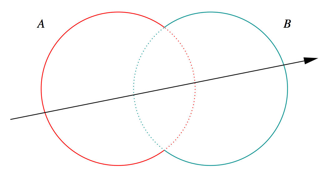
Constructive Solid Geometry (CSG) : Shapes defined "by construction"
Simple by construction definition, implicit geometry.
- A, B implicit primitive solids
- A + B : union (OR)
- A * B : intersection (AND)
- A - B : difference (AND NOT)
- !B : complement (NOT) (inside <-> outside)
CSG expressions
- non-unique: A - B == A * !B
- represented by binary tree, primitives at leaves
3D Parametric Ray : ray(t) = r0 + t rDir
Ray Geometry Intersection
- primitive : find t roots of implicit eqn
- composite : pick primitive intersect, depending on CSG tree
How to pick exactly ?
CSG : Which primitive intersect to pick ?
Classical Roth diagram approach
- find all ray/primitive intersects
- recursively combine inside intervals using CSG operator
- works from leaves upwards
Computational requirements:
- find all intersects, store them, order them
- recursive traverse
BUT : High performance on GPU requires:
- massive parallelism -> more the merrier
- low register usage -> keep it simple
- small stack size -> avoid recursion
Classical approach not appropriate on GPU
CSG Complete Binary Tree Serialization -> simplifies GPU side
CSG Tree, leaf node primitives, internal node operators, 4x4 transforms on any node,
serialized as complete binary tree:
- bit twiddling navigation avoids recursion
- no need to deserialize
- no child/parent pointers
- BUT: very inefficient when unbalanced
Height 3 complete binary tree with level order indices:
                                                   depth     elevation

                     1                               0           3

          10                   11                    1           2

     100       101        110        111             2           1

 1000 1001  1010 1011  1100 1101  1110  1111         3           0
postorder_next(i,elevation) = i & 1 ? i >> 1 : (i << elevation) + (1 << elevation) ; // from pattern of bits
Postorder tree traverse visits all nodes, starting from leftmost, such that children
are visited prior to their parents.
Evaluative CSG intersection Pseudocode : recursion emulated
fullTree = PACK( 1 << height, 1 >> 1 )  // leftmost, parent_of_root(=0)
tranche.push(fullTree, ray.tmin)

while (!tranche.empty)         // stack of begin/end indices
{
    begin, end, tmin <- tranche.pop  ; node <- begin ;
    while( node != end )                   // over tranche of postorder traversal
    {
        elevation = height - TREE_DEPTH(node) ;
        if(is_primitive(node)){ isect <- intersect_primitive(node, tmin) ;  csg.push(isect) }
        else{
            i_left, i_right = csg.pop, csg.pop            // csg stack of intersect normals, t
            l_state = CLASSIFY(i_left, ray.direction, tmin)
            r_state = CLASSIFY(i_right, ray.direction, tmin)
            action = LUT(operator(node), leftIsCloser)(l_state, r_state)

            if(      action is ReturnLeft/Right)     csg.push(i_left or i_right)
            else if( action is LoopLeft/Right)
            {
                left = 2*node ; right = 2*node + 1 ;
                endTranche = PACK( node,  end );
                leftTranche = PACK(  left << (elevation-1), right << (elevation-1) )
                rightTranche = PACK(  right << (elevation-1),  node  )
                loopTranche = action ? leftTranche : rightTranche

                tranche.push(endTranche, tmin)
                tranche.push(loopTranche, tminAdvanced )  // subtree re-traversal with changed tmin
                break ; // to next tranche
            }
        }
        node <- postorder_next(node, elevation)         // bit twiddling postorder
    }
}
isect = csg.pop();         // winning intersect
https://bitbucket.org/simoncblyth/opticks/src/tip/optixrap/cu/csg_intersect_boolean.h
Opticks CSG Primitives : Closed Solids, Consistent Normals
Closed Solid as: implementation requires otherside intersect, Rigidly attached normals
| Type code |
Python name |
C++ nnode sub-struct |
|---|
| CSG_BOX3,CSG_BOX |
box3,box |
nbox |
| CSG_SPHERE,CSG_ZSPHERE |
sphere,zsphere |
nsphere,nzsphere |
| CSG_CYLINDER,CSG_DISC |
cylinder,disc |
ncylinder,ndisc |
| CSG_CONE |
cone |
ncone |
| CSG_CONVEXPOLYHEDRON |
convexpolyhedron |
nconvexpolyhedron |
| CSG_TRAPEZOID,CSG_SEGMENT |
trapezoid,segment |
nconvexpolyhedron |
| CSG_TORUS |
torus |
ntorus |
| CSG_HYPERBOLOID |
hyperboloid |
nhyperboloid |
- zsphere, cone, cylinder, disc : truncated shapes closed by endcaps <-- NOT OPTIONAL
- disc : avoids endcap degeneracy with very thin cylinders
- convexpolyhedron : defined by a set of planes, used for trapezoid and segment
- segment : prism shape used for deltaphi intersection
- !complemented (inside<->outside) solids handled by
special casing classification (cannot miss otherside).
Non-primitives, high level CSG definition avoids loadsa code
- ellipsoid : non-uniform scaling of sphere, polycone : union of cylinders and cones
- inner-radii : via subtraction, deltaphi-segment : via intersect with segment
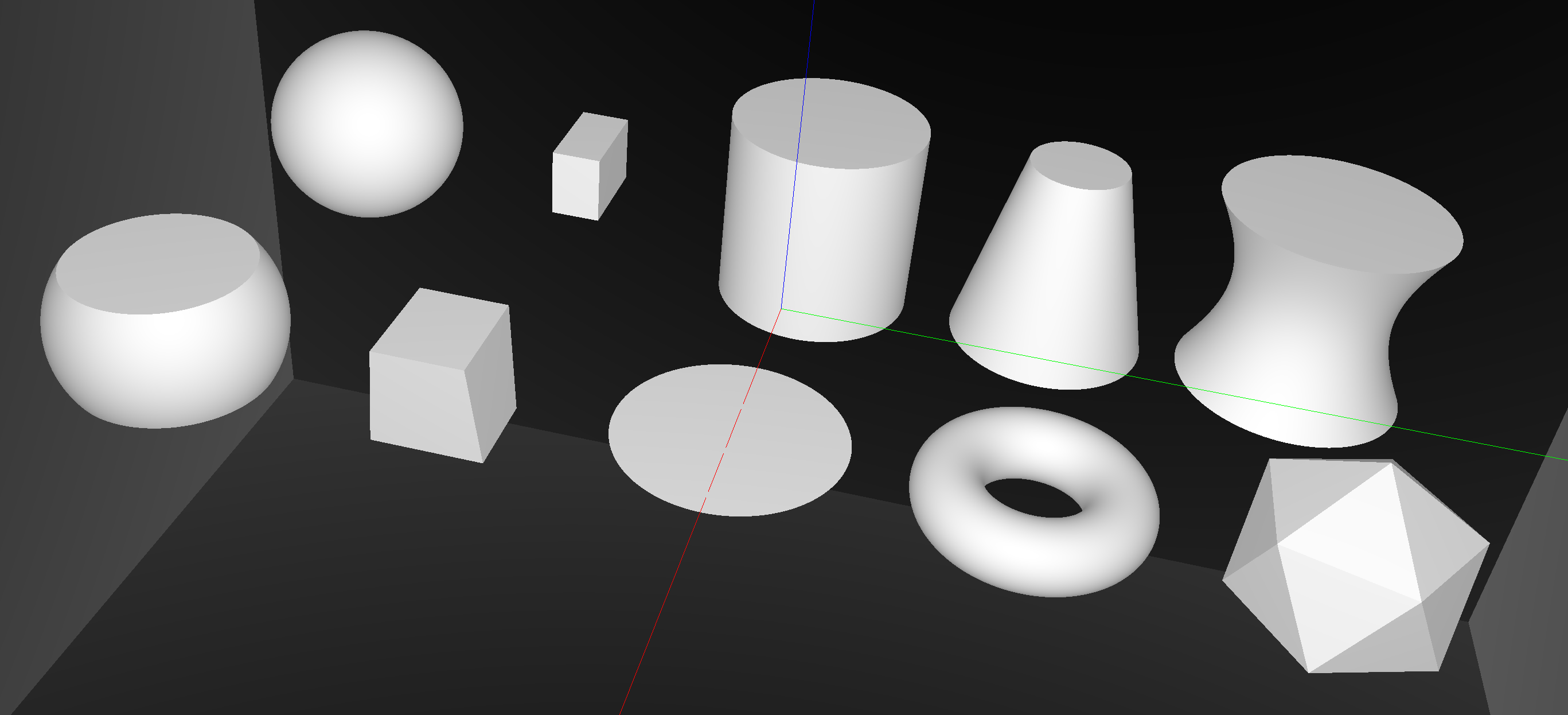
Opticks CSG Primitives : What is included
OptiX/CUDA functions providing:
- axis aligned bounding box (AABB)
- intersect ray position (parametric t), surface normal
C++/nnode sub-struct methods
- signed distance function (SDF)
- parametric surface generation
4x4 Transforms on any node (translation/rotation/scaling)
Intersect inverse-transformed ray with un-transformed primitive
- parametric-t same in both frames
- inverse transform transposed brings normal back to world frame
Supporting non-uniform scaling requires rayDir not be be normalized (or assumed to be normalized) by primitives.
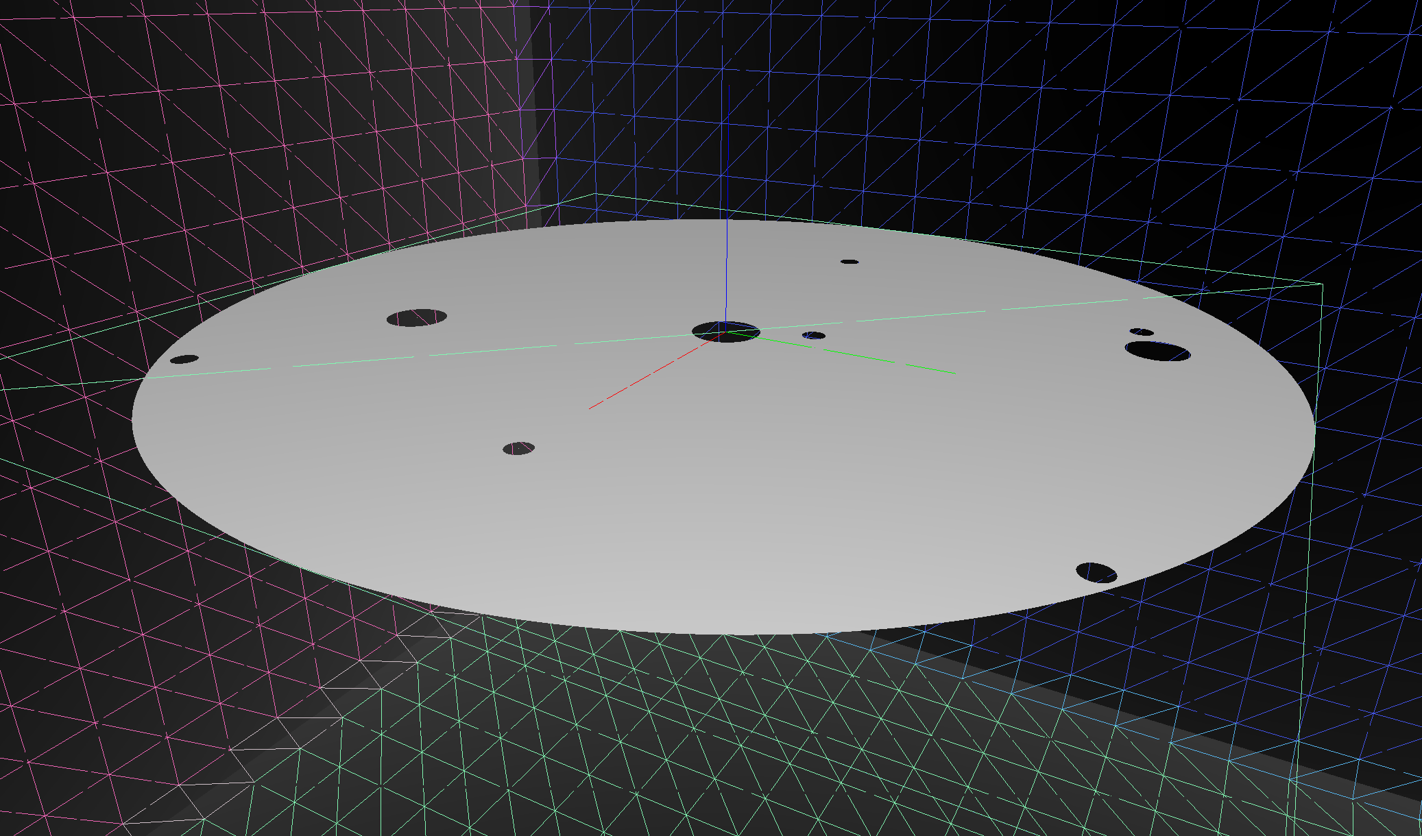
Dayabay ESR reflector : Deep CSG tree : disc with 9 holes
Opticks CSG Serialized into OpticksCSG format (numpy buffers, json)
// tboolean-parade

from opticks.ana.base import opticks_main
from opticks.analytic.csg import CSG

args = opticks_main(csgpath="$TMP/$FUNCNAME")

container = CSG("box", param=[0,0,0,1200], boundary=args.container, poly="MC", nx="20" )

a = CSG("sphere", param=[0,0,0,100])
b = CSG("zsphere", param=[0,0,0,100], param1=[-50,60,0,0])
c = CSG("box3",param=[100,50,70,0])
d = CSG.MakeTrapezoid(z=100, x1=80, y1=100, x2=100, y2=80)
e = CSG("cylinder",param=[0,0,0,100], param1=[-100,100,0,0])
f = CSG("disc",param=[0,0,0,100], param1=[-1,1,0,0])
g = CSG("cone", param=[100,-100,50,100])
h = CSG.MakeTorus(R=70, r=30)
i = CSG.MakeHyperboloid(r0=80, zf=100, z1=-100, z2=100)
j = CSG.MakeIcosahedron(scale=100.)

prims = [a,b,c,d,e,f,g,h,i,j]

...  // setting translations

CSG.Serialize([container] + prims, args.csgpath )     <-- write trees to file
- imported into C++ nnode tree by NCSG
tconcentric : spherical GdLS/LS/MineralOil
tconcentric : Opticks/Geant4 chi2 comparison
.      seqhis_ana  1:concentric   -1:concentric     c2
.                       1000000   1000000       373.13/356 =  1.05  (pval:0.256 prob:0.744)
0000           8ccccd    669843    670001             0.02  [6 ] TO BT BT BT BT SA
0001               4d     83950     84149             0.24  [2 ] TO AB
0002          8cccc6d     45490     44770             5.74  [7 ] TO SC BT BT BT BT SA
0003           4ccccd     28955     28718             0.97  [6 ] TO BT BT BT BT AB
0004             4ccd     23187     23170             0.01  [4 ] TO BT BT AB
0005          8cccc5d     20238     20140             0.24  [7 ] TO RE BT BT BT BT SA
0006          8cc6ccd     10214     10357             0.99  [7 ] TO BT BT SC BT BT SA
0007          86ccccd     10176     10318             0.98  [7 ] TO BT BT BT BT SC SA
0008          89ccccd      7540      7710             1.90  [7 ] TO BT BT BT BT DR SA
0009         8cccc55d      5976      5934             0.15  [8 ] TO RE RE BT BT BT BT SA
0010              45d      5779      5766             0.01  [3 ] TO RE AB
0011  8cccccccc9ccccd      5339      5269             0.46  [15] TO BT BT BT BT DR BT BT BT BT BT BT BT BT SA
0012          8cc5ccd      5111      4940             2.91  [7 ] TO BT BT RE BT BT SA
0013              46d      4797      4886             0.82  [3 ] TO SC AB
0014      8cccc9ccccd      4494      4469             0.07  [11] TO BT BT BT BT DR BT BT BT BT SA
0015      8cccccc6ccd      3317      3302             0.03  [11] TO BT BT SC BT BT BT BT BT BT SA
0016         8cccc66d      2670      2675             0.00  [8 ] TO SC SC BT BT BT BT SA
0017          49ccccd      2432      2383             0.50  [7 ] TO BT BT BT BT DR AB
0018          4cccc6d      2043      1991             0.67  [7 ] TO SC BT BT BT BT AB
0019            4cc6d      1755      1826             1.41  [5 ] TO SC BT BT AB
Top 20 chart above, (category 100 down to ~100 photons for propagation of 1M photons)
tconcentric : Opticks/Geant4 distrib chi2/df ~ 1.0
- Top 100 history categories correspond to ~900 propagation points
- 8 quantities at each point : ~7200 histograms pairs to chi2 compare
- selecting discrepant points : distchi2 > 1.1 (yields 41 out of 900 points)
XYZT:position/time ABCW:polarization/wavelength
| iv |
is |
na |
nb |
reclab |
X |
Y |
Z |
T |
A |
B |
C |
W |
seqc2 |
distc2 |
|---|
| 26 |
5 |
20238 |
20140 |
TO [RE] BT BT BT BT SA |
0.85 |
0.00 |
0.00 |
1.31 |
1.12 |
1.37 |
1.10 |
0.78 |
0.24 |
1.10 |
| 27 |
5 |
20238 |
20140 |
TO RE [BT] BT BT BT SA |
2.14 |
2.26 |
0.80 |
1.08 |
1.15 |
0.82 |
0.76 |
0.78 |
0.24 |
1.18 |
| 28 |
5 |
20238 |
20140 |
TO RE BT [BT] BT BT SA |
2.01 |
2.23 |
0.79 |
0.83 |
1.17 |
0.83 |
0.83 |
0.78 |
0.24 |
1.17 |
| 29 |
5 |
20238 |
20140 |
TO RE BT BT [BT] BT SA |
2.66 |
4.37 |
1.13 |
0.49 |
1.20 |
0.81 |
0.79 |
0.78 |
0.24 |
1.68 |
| 30 |
5 |
20238 |
20140 |
TO RE BT BT BT [BT] SA |
2.56 |
4.48 |
1.19 |
1.04 |
1.12 |
0.97 |
0.91 |
0.78 |
0.24 |
1.75 |
| 31 |
5 |
20238 |
20140 |
TO RE BT BT BT BT [SA] |
3.18 |
5.17 |
1.23 |
0.48 |
1.12 |
0.97 |
0.91 |
0.78 |
0.24 |
2.06 |
| 38 |
6 |
10214 |
10357 |
TO BT BT SC BT BT [SA] |
0.79 |
1.37 |
1.43 |
0.55 |
1.00 |
1.33 |
0.97 |
0.00 |
0.99 |
1.16 |
| 52 |
8 |
7540 |
7710 |
TO BT BT BT BT DR [SA] |
1.70 |
1.32 |
1.48 |
1.49 |
1.12 |
1.03 |
1.37 |
0.00 |
1.90 |
1.28 |
| 56 |
9 |
5976 |
5934 |
TO RE RE [BT] BT BT BT SA |
1.26 |
1.51 |
1.21 |
2.36 |
0.99 |
1.40 |
1.10 |
1.65 |
0.15 |
1.24 |
| 57 |
9 |
5976 |
5934 |
TO RE RE BT [BT] BT BT SA |
1.23 |
1.39 |
1.25 |
2.31 |
0.98 |
1.45 |
0.98 |
1.65 |
0.15 |
1.21 |
| 58 |
9 |
5976 |
5934 |
TO RE RE BT BT [BT] BT SA |
1.24 |
0.98 |
1.18 |
1.88 |
0.97 |
1.39 |
1.01 |
1.65 |
0.15 |
1.14 |
| 59 |
9 |
5976 |
5934 |
TO RE RE BT BT BT [BT] SA |
1.24 |
0.90 |
1.04 |
1.83 |
0.93 |
1.55 |
0.92 |
1.65 |
0.15 |
1.11 |
| 60 |
9 |
5976 |
5934 |
TO RE RE BT BT BT BT [SA] |
0.95 |
1.03 |
1.50 |
3.12 |
0.93 |
1.55 |
0.92 |
1.65 |
0.15 |
1.18 |
| 69 |
11 |
5339 |
5269 |
TO BT BT BT BT [DR] BT BT BT BT BT BT BT BT SA |
0.00 |
0.00 |
0.00 |
0.00 |
1.29 |
1.69 |
2.42 |
0.00 |
0.46 |
1.31 |
| 74 |
11 |
5339 |
5269 |
TO BT BT BT BT DR BT BT BT BT [BT] BT BT BT SA |
1.10 |
1.45 |
1.02 |
0.67 |
1.42 |
0.83 |
1.38 |
0.00 |
0.46 |
1.12 |
| 75 |
11 |
5339 |
5269 |
TO BT BT BT BT DR BT BT BT BT BT [BT] BT BT SA |
0.98 |
1.42 |
1.16 |
0.52 |
1.58 |
0.82 |
1.46 |
0.00 |
0.46 |
1.15 |
| 76 |
11 |
5339 |
5269 |
TO BT BT BT BT DR BT BT BT BT BT BT [BT] BT SA |
1.46 |
1.66 |
0.79 |
0.65 |
1.69 |
0.89 |
1.46 |
0.00 |
0.46 |
1.21 |
| 77 |
11 |
5339 |
5269 |
TO BT BT BT BT DR BT BT BT BT BT BT BT [BT] SA |
1.04 |
1.64 |
0.81 |
0.51 |
2.20 |
0.91 |
1.35 |
0.00 |
0.46 |
1.19 |
| 78 |
11 |
5339 |
5269 |
TO BT BT BT BT DR BT BT BT BT BT BT BT BT [SA] |
1.10 |
1.56 |
0.73 |
0.21 |
2.20 |
0.91 |
1.35 |
0.00 |
0.46 |
1.17 |
| 85 |
12 |
5111 |
4940 |
TO BT BT RE BT BT [SA] |
1.26 |
2.13 |
0.79 |
2.07 |
1.03 |
0.93 |
0.72 |
0.68 |
2.91 |
1.11 |
| 94 |
14 |
4494 |
4469 |
TO BT BT BT BT [DR] BT BT BT BT SA |
0.00 |
0.00 |
0.00 |
0.00 |
1.90 |
3.74 |
1.95 |
0.00 |
0.07 |
2.01 |
| 95 |
14 |
4494 |
4469 |
TO BT BT BT BT DR [BT] BT BT BT SA |
3.85 |
1.83 |
0.90 |
0.82 |
2.20 |
1.45 |
1.11 |
0.00 |
0.07 |
1.41 |
| 96 |
14 |
4494 |
4469 |
TO BT BT BT BT DR BT [BT] BT BT SA |
1.94 |
1.82 |
1.07 |
0.85 |
2.67 |
1.30 |
1.08 |
0.00 |
0.07 |
1.39 |
| 97 |
14 |
4494 |
4469 |
TO BT BT BT BT DR BT BT [BT] BT SA |
1.61 |
1.35 |
1.48 |
0.31 |
2.00 |
1.22 |
1.28 |
0.00 |
0.07 |
1.35 |
| 98 |
14 |
4494 |
4469 |
TO BT BT BT BT DR BT BT BT [BT] SA |
1.96 |
1.31 |
1.39 |
0.66 |
2.13 |
1.03 |
1.42 |
0.00 |
0.07 |
1.36 |
| 99 |
14 |
4494 |
4469 |
TO BT BT BT BT DR BT BT BT BT [SA] |
2.29 |
0.91 |
1.05 |
4.14 |
2.13 |
1.03 |
1.42 |
0.00 |
0.07 |
1.23 |
| 104 |
15 |
3317 |
3302 |
TO BT BT SC [BT] BT BT BT BT BT SA |
0.60 |
1.02 |
1.75 |
1.92 |
0.77 |
1.23 |
1.39 |
0.00 |
0.03 |
1.20 |
| 105 |
15 |
3317 |
3302 |
TO BT BT SC BT [BT] BT BT BT BT SA |
0.77 |
1.35 |
1.34 |
1.98 |
0.73 |
1.13 |
1.41 |
0.00 |
0.03 |
1.17 |
| 108 |
15 |
3317 |
3302 |
TO BT BT SC BT BT BT BT [BT] BT SA |
1.48 |
1.01 |
1.73 |
0.51 |
0.85 |
1.00 |
1.05 |
0.00 |
0.03 |
1.15 |
| 124 |
17 |
2432 |
2383 |
TO BT BT BT BT [DR] AB |
0.00 |
0.00 |
0.00 |
0.00 |
1.64 |
0.92 |
0.71 |
0.00 |
0.50 |
1.20 |
| 140 |
20 |
1815 |
1805 |
TO RE [RE] RE BT BT BT BT SA |
1.80 |
0.56 |
1.73 |
0.59 |
1.31 |
1.20 |
1.42 |
0.60 |
0.03 |
1.26 |
| 141 |
20 |
1815 |
1805 |
TO RE RE [RE] BT BT BT BT SA |
1.30 |
1.02 |
2.24 |
1.02 |
1.09 |
1.06 |
1.17 |
1.07 |
0.03 |
1.15 |
| 144 |
20 |
1815 |
1805 |
TO RE RE RE BT BT [BT] BT SA |
1.05 |
1.32 |
1.03 |
0.53 |
0.93 |
1.31 |
1.12 |
1.07 |
0.03 |
1.10 |
| 222 |
29 |
1105 |
1168 |
TO BT BT RE BT BT [BT] BT BT BT SA |
2.42 |
2.53 |
2.26 |
2.49 |
1.29 |
1.25 |
0.65 |
1.08 |
1.75 |
1.65 |
| 223 |
29 |
1105 |
1168 |
TO BT BT RE BT BT BT [BT] BT BT SA |
2.32 |
2.44 |
1.98 |
2.38 |
1.03 |
1.07 |
0.72 |
1.08 |
1.75 |
1.53 |
| 224 |
29 |
1105 |
1168 |
TO BT BT RE BT BT BT BT [BT] BT SA |
3.13 |
2.49 |
1.32 |
1.34 |
1.11 |
1.23 |
0.69 |
1.08 |
1.75 |
1.56 |
| 225 |
29 |
1105 |
1168 |
TO BT BT RE BT BT BT BT BT [BT] SA |
2.83 |
2.44 |
1.36 |
1.06 |
0.92 |
1.08 |
0.69 |
1.08 |
1.75 |
1.47 |
| 226 |
29 |
1105 |
1168 |
TO BT BT RE BT BT BT BT BT BT [SA] |
3.24 |
3.21 |
1.03 |
2.18 |
0.92 |
1.08 |
0.69 |
1.08 |
1.75 |
1.59 |
| 241 |
31 |
1067 |
1013 |
TO BT BT BT BT DR [BT] BT AB |
1.25 |
1.53 |
0.80 |
0.27 |
2.03 |
0.90 |
1.40 |
0.00 |
1.40 |
1.27 |
| 242 |
31 |
1067 |
1013 |
TO BT BT BT BT DR BT [BT] AB |
1.30 |
1.88 |
0.76 |
0.37 |
1.44 |
0.95 |
1.38 |
0.00 |
1.40 |
1.18 |
| 248 |
32 |
1036 |
988 |
TO RE BT BT [AB] |
1.00 |
1.78 |
1.69 |
1.55 |
0.62 |
0.87 |
0.86 |
1.33 |
1.14 |
1.13 |
PMT Opticks/Geant4 step distribution comparison TO BT [SD]
Good agreement reached, after several fixes: geometry, total internal reflection, group velocity
PMT Opticks/Geant4 step distribution comparison : chi2/ndf
| 4/PMT In Box/torch : |
X |
Y |
Z |
T |
A |
B |
C |
R |
|---|
| 340271/340273 : [TO] BT SA |
1.15 |
1.00 |
0.00 |
0.00 |
1.06 |
1.03 |
0.00 |
1.21 |
| 340271/340273 : TO [BT] SA |
1.15 |
1.00 |
1.06 |
0.91 |
1.06 |
1.03 |
0.00 |
1.21 |
| 340271/340273 : TO BT [SA] |
0.97 |
1.02 |
1.05 |
0.99 |
1.06 |
1.03 |
0.00 |
1.29 |
| 107598/107251 : [TO] BT SD |
0.91 |
0.73 |
0.56 |
0.56 |
0.98 |
1.09 |
0.56 |
0.94 |
| 107598/107251 : TO [BT] SD |
0.91 |
0.73 |
0.81 |
0.93 |
0.98 |
1.09 |
0.56 |
0.94 |
| 107598/107251 : TO BT [SD] |
0.99 |
0.83 |
0.97 |
0.99 |
0.98 |
1.09 |
0.56 |
0.93 |
| 23217/23260 : [TO] BT BT SA |
0.94 |
0.82 |
0.04 |
0.04 |
0.97 |
0.89 |
0.04 |
0.57 |
| 23217/23260 : TO [BT] BT SA |
0.94 |
0.82 |
0.70 |
0.50 |
0.97 |
0.89 |
0.04 |
0.57 |
| 23217/23260 : TO BT [BT] SA |
0.91 |
0.94 |
0.43 |
0.60 |
0.97 |
0.89 |
0.04 |
0.05 |
| 23217/23260 : TO BT BT [SA] |
0.94 |
0.88 |
0.04 |
0.35 |
0.97 |
0.89 |
0.04 |
0.72 |
| 18866/19048 : [TO] AB |
0.99 |
1.10 |
0.87 |
0.87 |
0.85 |
0.84 |
0.87 |
1.00 |
| 18866/19048 : TO [AB] |
0.99 |
1.10 |
0.93 |
0.92 |
0.85 |
0.84 |
0.87 |
1.00 |
| 3179/3133 : [TO] SC SA |
1.07 |
0.83 |
0.34 |
0.34 |
0.86 |
0.96 |
0.34 |
0.73 |
| 3179/3133 : TO [SC] SA |
1.07 |
0.83 |
0.98 |
1.05 |
0.98 |
1.06 |
0.98 |
0.73 |
| 3179/3133 : TO SC [SA] |
0.96 |
1.04 |
0.93 |
0.97 |
0.98 |
1.06 |
0.98 |
1.10 |
| 2204/2249 : [TO] BT AB |
0.85 |
1.04 |
0.45 |
0.45 |
0.99 |
0.92 |
0.45 |
1.06 |
| 2204/2249 : TO [BT] AB |
0.85 |
1.04 |
0.95 |
0.88 |
0.99 |
0.92 |
0.45 |
1.06 |
| 2204/2249 : TO BT [AB] |
0.98 |
0.94 |
1.01 |
1.00 |
0.99 |
0.92 |
0.45 |
0.90 |
| 1696/1732 : [TO] BT BT AB |
1.05 |
0.85 |
0.38 |
0.38 |
0.86 |
1.09 |
0.38 |
0.26 |
| 1696/1732 : TO [BT] BT AB |
1.05 |
0.85 |
1.48 |
1.28 |
0.86 |
1.09 |
0.38 |
0.26 |
| 1696/1732 : TO BT [BT] AB |
0.99 |
0.86 |
1.17 |
1.40 |
0.86 |
1.09 |
0.38 |
0.86 |
| 1696/1732 : TO BT BT [AB] |
1.15 |
0.88 |
1.08 |
1.06 |
0.86 |
1.09 |
0.38 |
0.79 |
| 1446/1455 : [TO] BR SA |
1.21 |
0.94 |
0.03 |
0.03 |
0.90 |
0.87 |
0.03 |
1.09 |
| 1446/1455 : TO [BR] SA |
1.21 |
0.94 |
1.02 |
1.01 |
0.90 |
0.87 |
0.03 |
1.09 |
| 1446/1455 : TO BR [SA] |
1.00 |
0.93 |
0.97 |
0.99 |
0.90 |
0.87 |
0.03 |
1.04 |
Opticks/Geant4 Rainbow Step Sequence Comparison
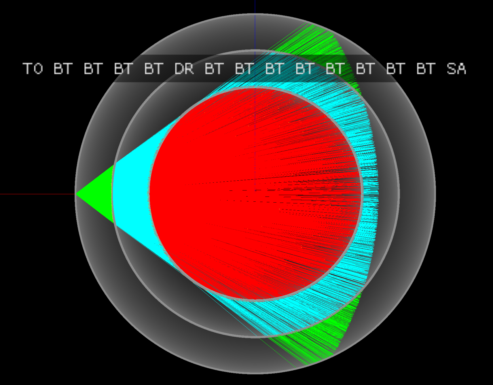
- Flags:
- BT/BR: boundary transmit/reflect
- TO/SC/SA: torch/scatter/surface absorb
Statistically consistent photon histories in the two simulations : Multiple orders of rainbow apparent
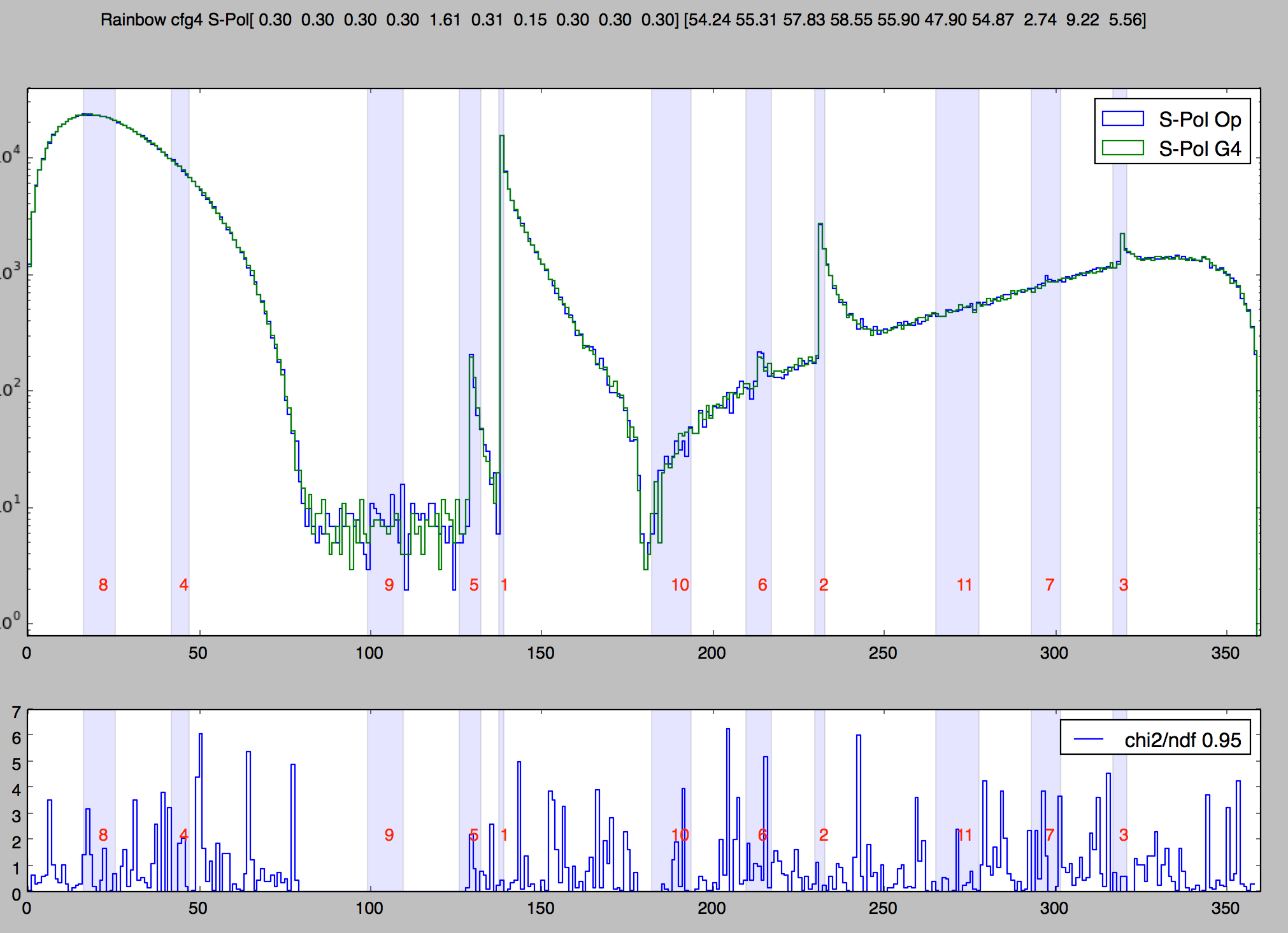
 64-bit uint  Opticks    Geant4    chi2                                      (tag:5,-5)

        8ccd   819160    819654    0.15  [4 ] TO BT BT SA                    (cross droplet)
         8bd   102087    101615    1.09  [3 ] TO BR SA                       (external reflect)
       8cbcd    61869     61890    0.00  [5 ] TO BT BR BT SA                 (bow 1)
      8cbbcd     9618      9577    0.09  [6 ] TO BT BR BR BT SA              (bow 2)
     8cbbbcd     2604      2687    1.30  [7 ] TO BT BR BR BR BT SA           (bow 3)
    8cbbbbcd     1056      1030    0.32  [8 ] TO BT BR BR BR BR BT SA        (bow 4)
       86ccd     1014      1000    0.10  [5 ] TO BT BT SC SA
   8cbbbbbcd      472       516    1.96  [9 ] TO BT BR BR BR BR BR BT SA     (bow 5)
         86d      498       473    0.64  [3 ] TO SC SA
  bbbbbbbbcd      304       294    0.17  [10] TO BT BR BR BR BR BR BR BR BR  (bow 8+ truncated)
  8cbbbbbbcd      272       247    1.20  [10] TO BT BR BR BR BR BR BR BT SA  (bow 6)
  cbbbbbbbcd      183       161    1.41  [10] TO BT BR BR BR BR BR BR BR BT  (bow 7 truncated)
1M Rainbow S-Polarized, Comparison Opticks/Geant4
Deviation angle(degrees) of 1M parallel monochromatic photons in disc shaped beam incident on water sphere.
Numbered bands are visible range expectations of first 11 rainbows.
S-Polarized intersection (E field perpendicular to plane of incidence) arranged by directing polarization radially.
Compare Opticks/Geant4 Simulations with Simple Lights/Geometries

- Photon step records
- 128 bit per step : highly compressed position, time, wavelength, polarization vector, material/history codes
- Photon flag sequence
- 16x 4-bit step flags recorded in uint64 sequence, indexed using Thrust GPU sort (1M indexed ~0.040s)
Sequence index -> interactive OpenGL selection of photons by flag sequence
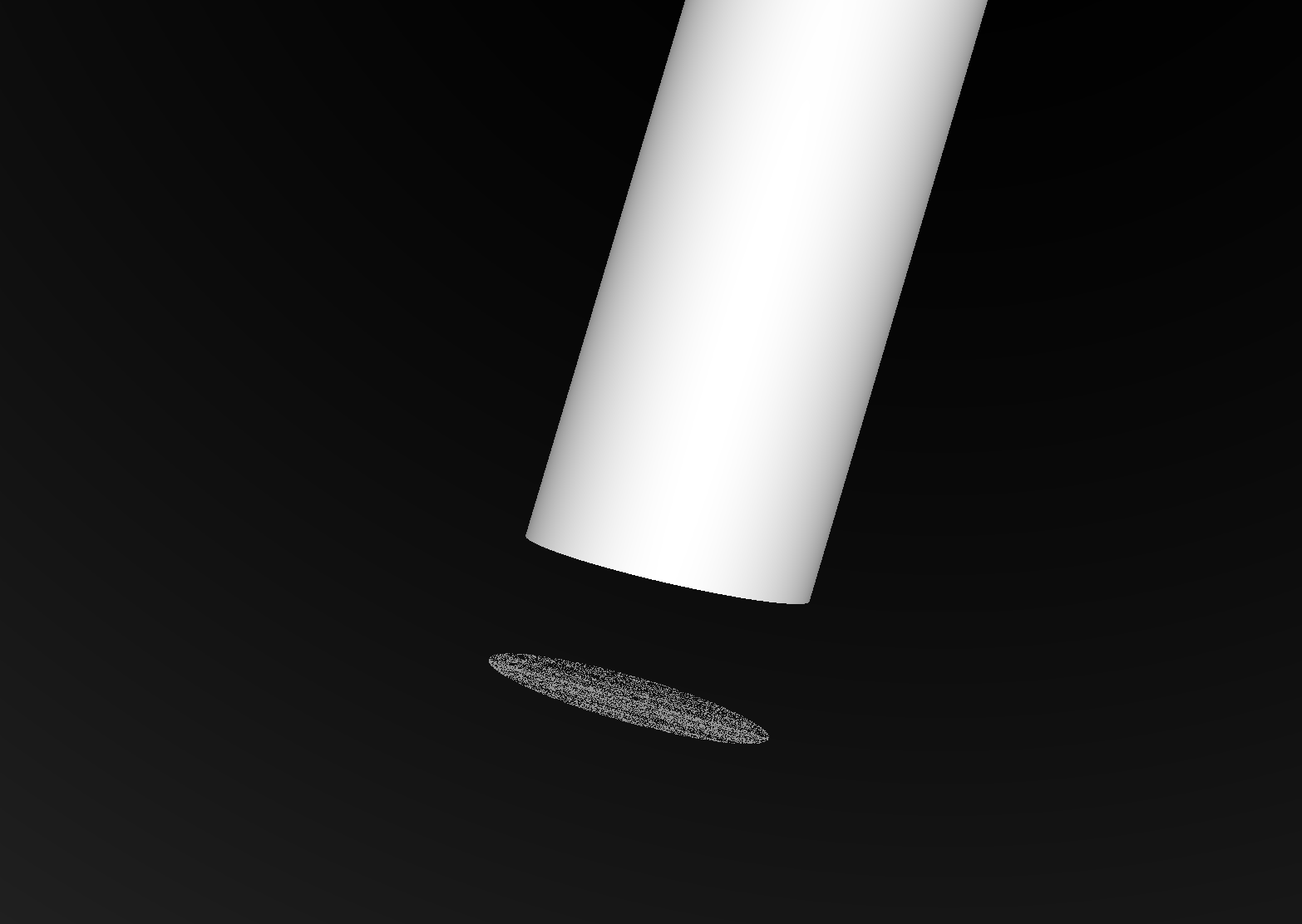
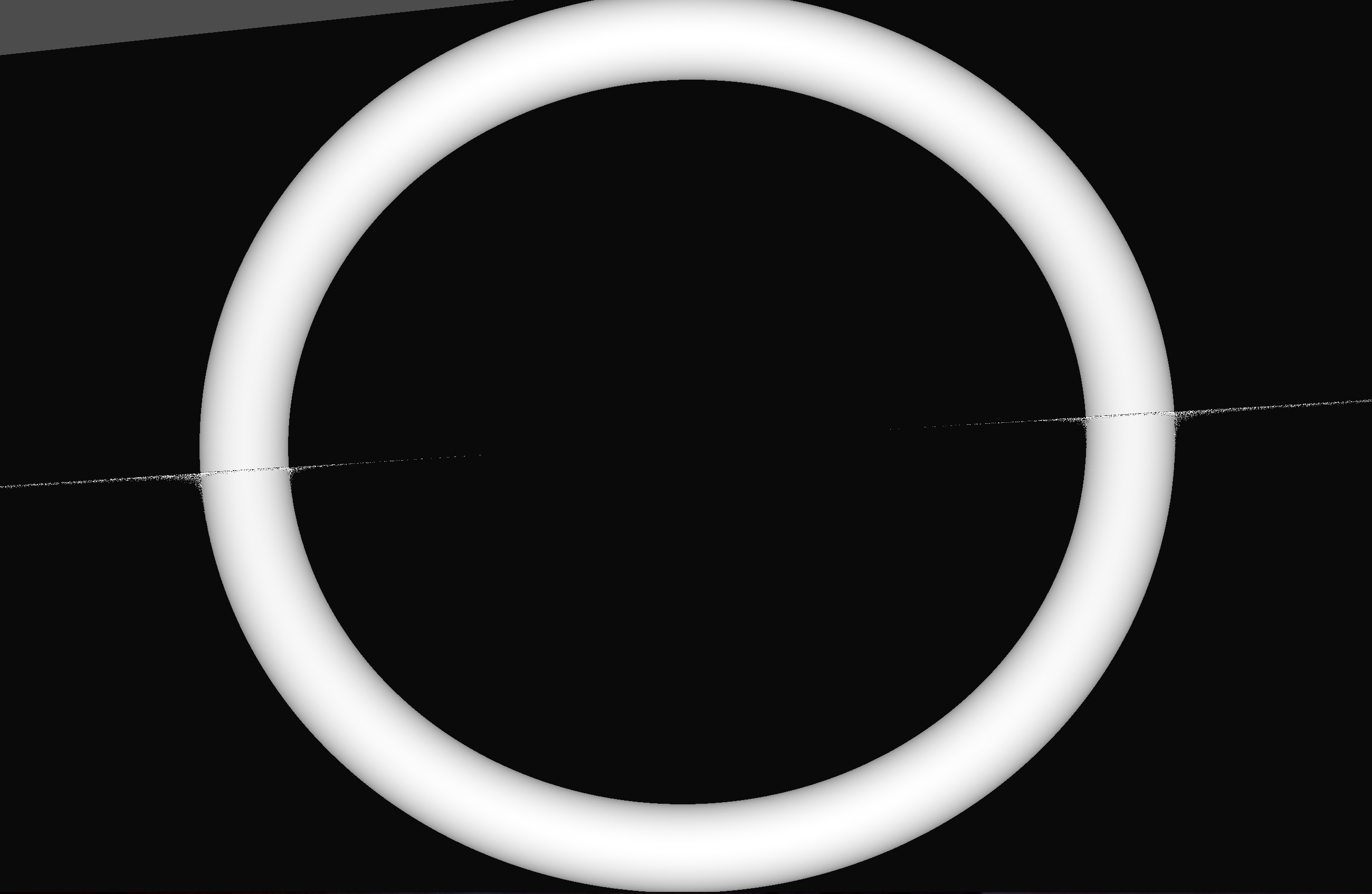
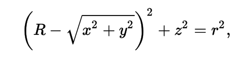
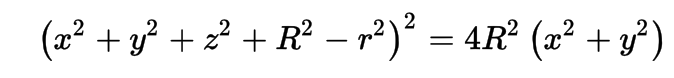
Torus : much more difficult/expensive than other primitives
3D parametric ray : ray(x,y,z;t) = rayOrigin + t * rayDirection
- ray-torus intersection -> solve quartic polynomial in t
- A t^4 + B t^3 + C t^2 + D t + E = 0
High order equation
- very large difference between coefficients
- varying ray -> wide range of very coefficients
- numerically problematic, requires double precision
- several mathematical approaches used, work in progress
Best Solution : replace torus
- eg model PMT neck with hyperboloid, not cylinder-torus
Geometry Modelling : Tesselated vs Analytic Photomultiplier Tubes
Analytic : more realistic, faster, less memory, much more effort
For Dayabay PMT:
- partition CSG solids into 12 single primitive parts (instead of 2928 triangles)
- splitting at geometrical intersections avoids implementing general CSG boolean handling
- geometry provided to OptiX in form of ray intersection and bounding box code
Aim : analytic description of geometry on critical optical path, remainder tesselated
OpticksDocs
NVIDIA OptiX 1
NVIDIA OptiX 2
https://research.nvidia.com/publication/optix-general-purpose-ray-tracing-engine
Ray intersection with general CSG binary tree solids within OptiX
Performance on GPU requires
- massive parallelism -> more the merrier
- low register usage -> keep it simple
- small stack size -> avoid recursion : OptiX demands: no recursion in intersect
Approach (details in backup)
- Complete Binary Tree Serialization
- postorder tree traversal, just by bit twiddling (avoids recursion)
- Ray Tracing CSG Objects Using Single Hit Intersections (A. Kensler)[1]
- binary intersect classification, lookup table
- avoids lots of state, BUT: sometimes advance t_min and re-intersect
- converted recursive pseudocode into "Evaluative" implementation [2]
- Auto translation of GDML into GPU appropriate form
- entire geometry translated, serialized, uploaded to GPU
- [1] Ray Tracing CSG Objects Using Single Hit Intersections, Andrew Kensler (2006)
- with corrections by author of XRT Raytracer http://xrt.wikidot.com/doc:csg
[2] Similar to binary expression tree evaluation using postorder traverse.
Opticks Analytic JUNO PMT Snap, GPU Raytrace (1)
GPU Instance Culling with Level Of Detail
Large Geometry Techniques : Instancing Mandatory
Geometry analysed to find repeats
JUNO: 18k 20" PMTs, 36k 3" PMTs
Instances used by:
- OptiX geometry
- OptiX acceleration structures
- OpenGL visualization
Advantages
- drastic reduction in GPU memory
- one set of vertices for each PMT type
- 4x4 matrices position each PMT
Viz Optimizations (OpenGL 4+)
Use geometry shader transform feedback:
- cull non-visible instances
- level of detail (LOD) meshes
- switch mesh based on distance to PMT
Opticks : Whats New ?
Geometry Handling
- General CSG boolean geometry intersection on GPU
- Geant4 geometry auto-translated to GPU without approximation
- Geometry direct from Geant4, no export/import needed
- Export Geant4 geometry to glTF 2.0 for visualization
Validation
- make any solid emit CPU generated "input" photons
- random sequence aligned validations
Configuration
- Modern CMake 3.5 target export -> easy integration with your code
Community
Opticks Analytic Daya Bay Near Site, GPU Raytrace (0)