Outline : Tools, Techniques and Opticks
- Introducing the Tools
- GPU, CUDA, Thrust
- NumPy
- Techniques
- Monte Carlo Method
- Geant4
- Opticks : Optical Photon Simulation
- problem, solution
- geometry, validation
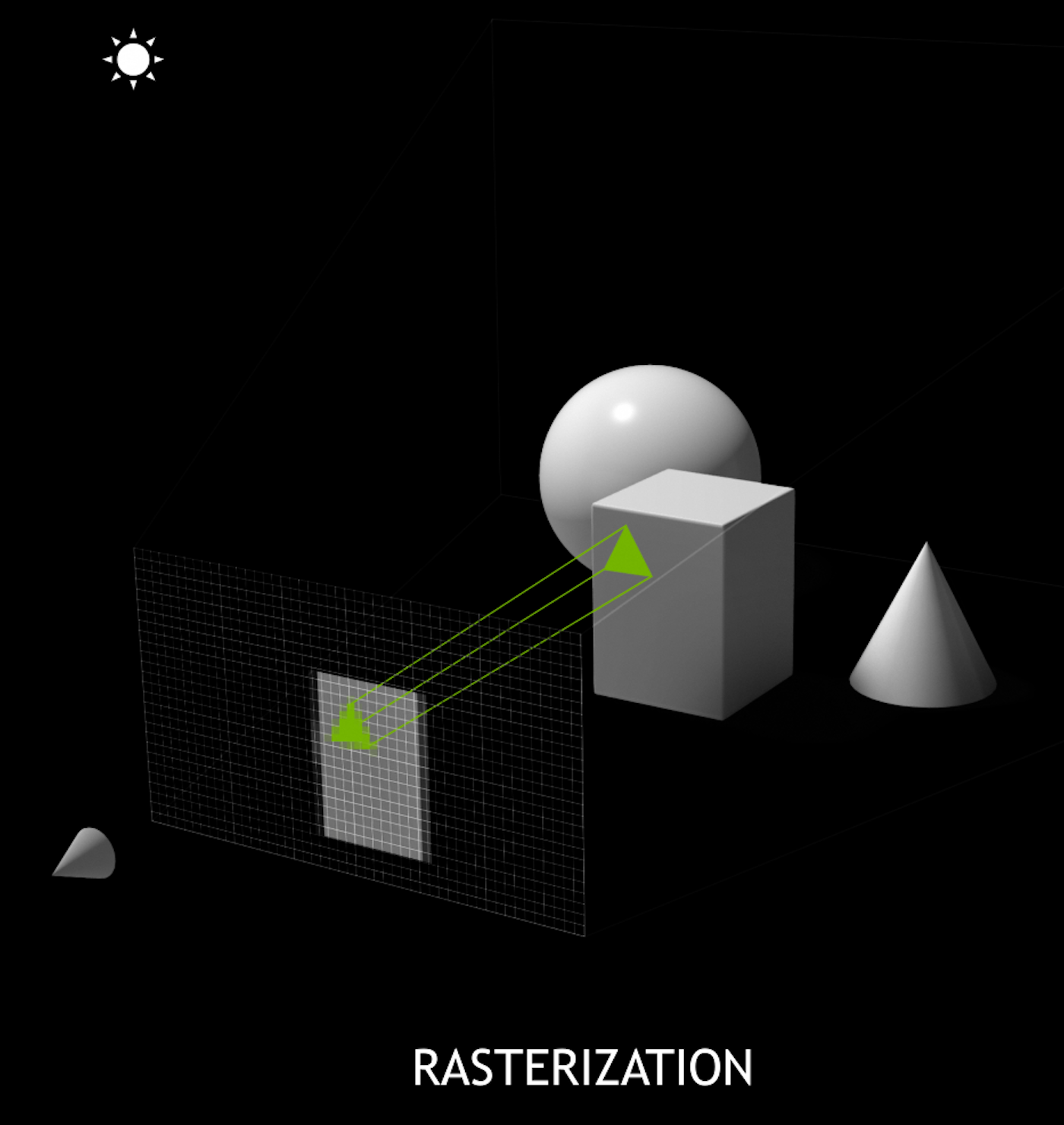
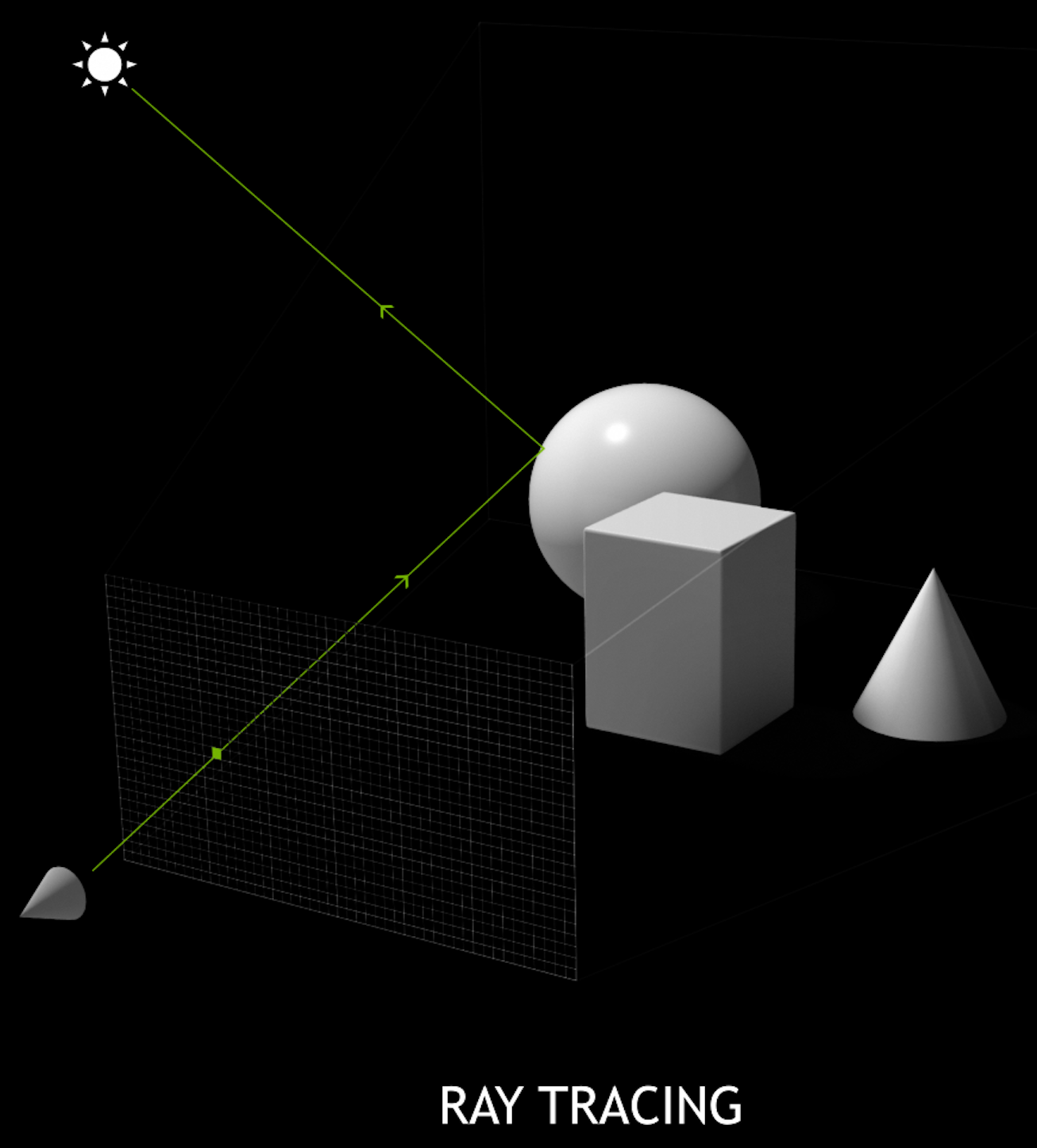
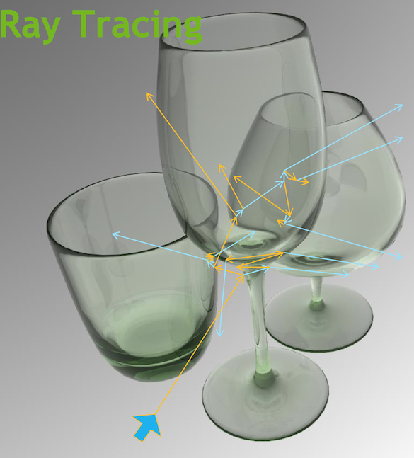
Ray-tracing vs Rasterization
Outline : Introducing the Tools
- Understanding GPUs
- Graphical Origins
- NVIDIA Turing GPU
- CPU vs GPU architectures
- Latency vs Throughput
- How to Make Effective Use of GPUs ?
- Use Higher Level Libraries -> Thrust
- Parallel / Simple / Uncoupled
- GPU Constraints -> Array-Oriented Design -> NumPy
- Serialization
- Serialization Benefits
- NumPy
- Foundation of Python Data Ecosystem
- Python : fastest growing major programming language ? Why ?
- NumPy Example : closest approach of Ellipse to a Circle
- NumPy Example : NLL Reconstruction fit : On one slide
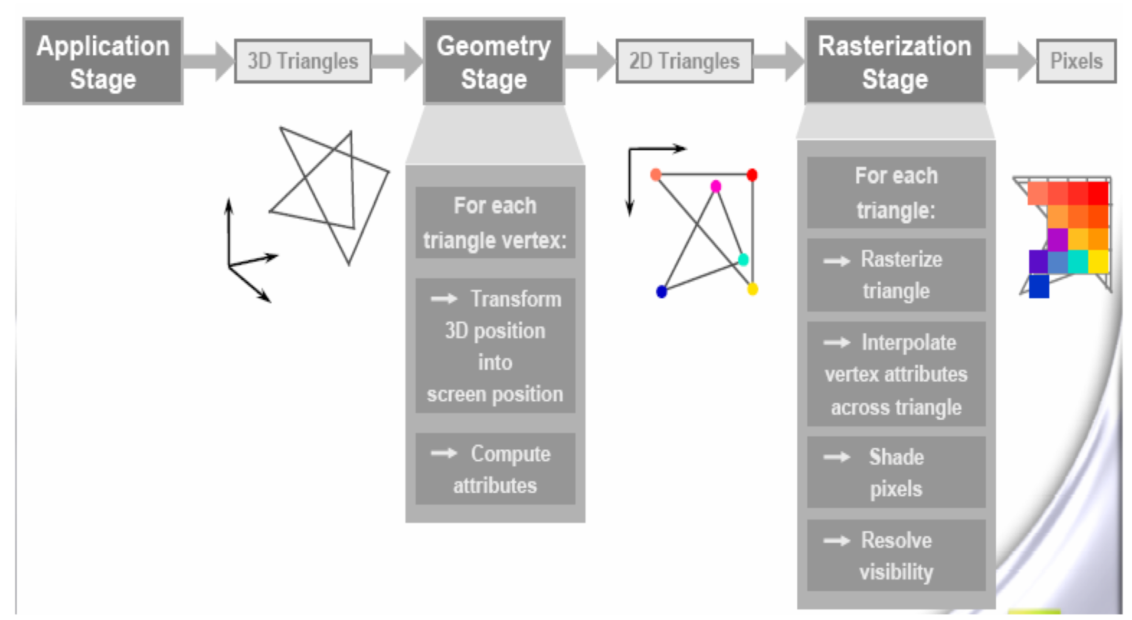
Understanding GPUs : Graphical Origins : An Extremely Parallel Problem
- GPUs evolved to rasterize 3D graphics, eg OpenGL graphics pipeline
- millions of triangles, millions of pixels, mostly independent
- simple data structures : vertices, triangles, pixels
- literally billions of small "shader" programs run per second
CPU vs GPU architectures, Latency vs Throughput
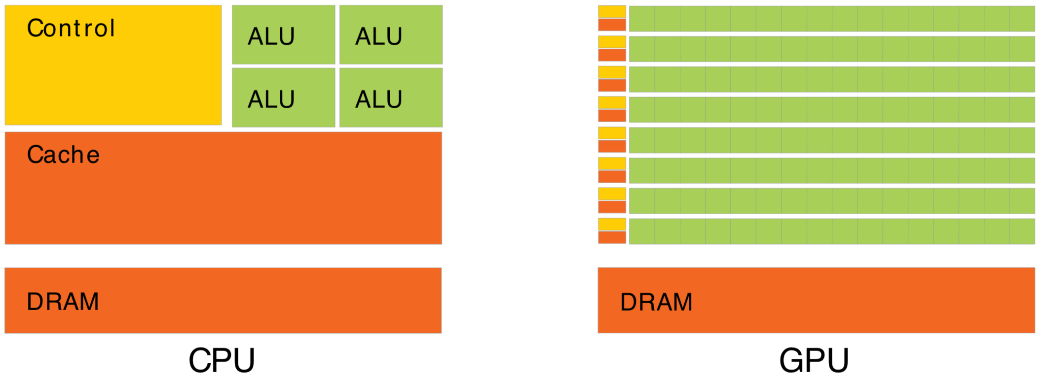
Waiting for memory read/write, is major source of latency...
- CPU : latency-oriented : Minimize time to complete single task : avoid latency with caching
- complex : caching system, branch prediction, speculative execution, ...
- GPU : throughput-oriented : Maximize total work per unit time : hide latency with parallelism
- many simple processing cores, hardware multithreading, SIMD (single instruction multiple data)
- simpler : lots of compute (ALU), at expense of cache+control
- design assumes abundant parallelism
Effective use of Totally different processor architecture -> Total reorganization of data and computation
Understanding Throughput-oriented Architectures https://cacm.acm.org/magazines/2010/11/100622-understanding-throughput-oriented-architectures/fulltext
How to Make Effective Use of GPUs ? -> Use Higher Level Libraries
"... Code at the speed of light ..."
"... high-level interface greatly enhances programmer productivity ..."
- https://developer.nvidia.com/Thrust
- header only library, comes with CUDA
- high-level abstraction : reduce, scan, sort
- rapid prototyping
- easy interop with CUDA
- Not many available, use if possible
- benefit from other peoples experience
- Thrust : high level C++ interface to CUDA
- OptiX : raytrace engine
- cuRAND, cuFFT, cuBLAS, cuSOLVER, ...
- CUB : http://nvlabs.github.io/cub/
https://developer.nvidia.com/gpu-accelerated-libraries

For adventurous early adopters
How to Make Effective Use of GPUs ? Parallel / Simple / Uncoupled
- Abundant parallelism
- many thousands of tasks (ideally millions)
- Low register usage : otherwise limits concurrent threads
- simple kernels, avoid branching
- Little/No Synchronization
- avoid waiting, avoid complex code/debugging
- Minimize CPU<->GPU copies
- reuse GPU buffers across multiple CUDA launches
How Many Threads to Launch ?
- can (and should) launch many millions of threads
- mince problems as finely as feasible
- maximum thread launch size : so large its irrelevant
- maximum threads inflight : #SM*2048 = 80*2048 ~ 160k
- best latency hiding when launch > ~10x this ~ 1M
Understanding Throughput-oriented Architectures https://cacm.acm.org/magazines/2010/11/100622-understanding-throughput-oriented-architectures/fulltext
NVIDIA Titan V: 80 SM, 5120 CUDA cores
NumPy : Foundation of Python Data Ecosystem
https://bitbucket.org/simoncblyth/intro_to_numpy
Very terse, array-oriented (no-loop) python interface to C performance
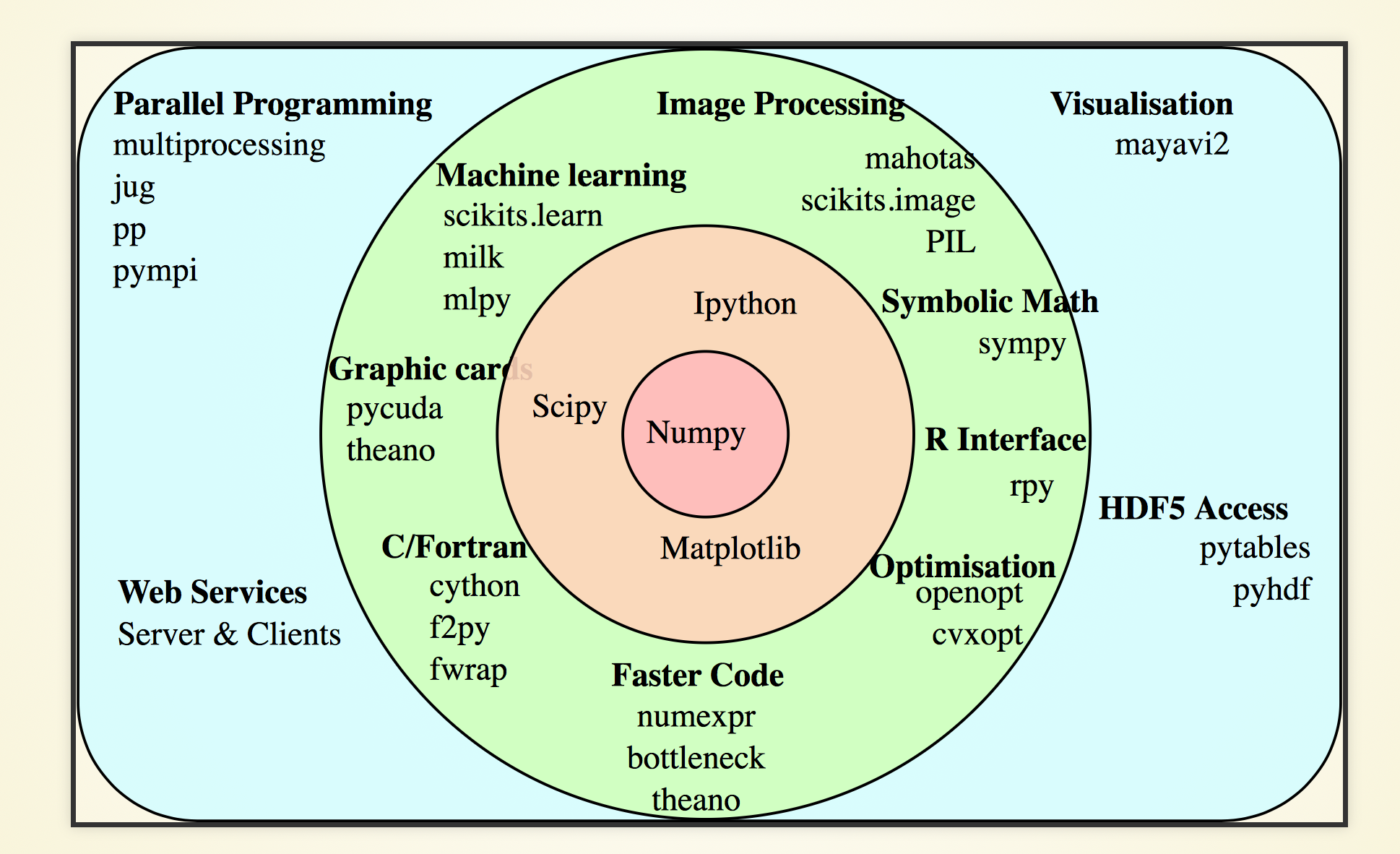
- C speed, python brevity + ease
- array-oriented
- vectorized : no python loops
- efficiently work with large arrays
- Recommended paper:
- The NumPy array: a structure for efficient numerical computation https://hal.inria.fr/inria-00564007
https://docs.scipy.org/doc/numpy/user/quickstart.html
http://www.scipy-lectures.org/intro/index.html
https://github.com/donnemartin/data-science-ipython-notebooks
Python : fastest growing major programming language : Why?
- Python more than doubled userbase over past five years (measured by Stackoverflow questions)
- Data science + machine learning developers prefer Python ? But why ?
- easy to learn, fast to write, fast to read
- efficient (no-copy) memory sharing between C/C++ libraries and scripts, due to Buffer Protocol
- easiest way to use Buffer Protocol (from Python and C) is via NumPy : so they all do:
- TensorFlow, Theano, Keras, Scikit-learn
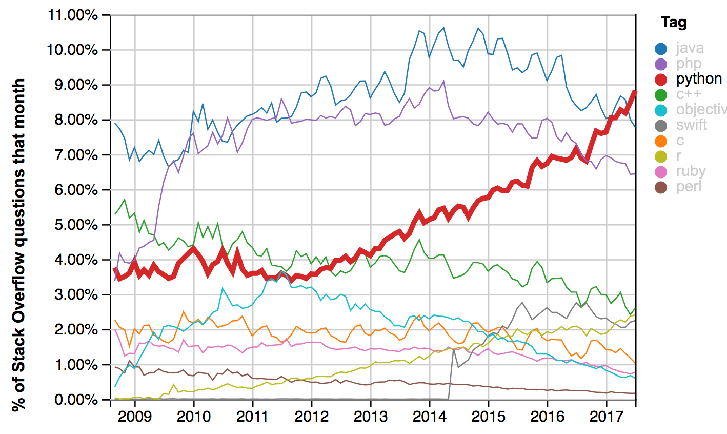
https://stackoverflow.blog/2017/09/14/python-growing-quickly/
https://insights.stackoverflow.com/trends
https://jakevdp.github.io/blog/2014/05/05/introduction-to-the-python-buffer-protocol/
Outline of Techniques : Monte Carlo Method
- Technique : Monte Carlo Method
- apply randomness to model complex systems
- optical photon simulation, deciding history
- sampling using Cumulative Distribution Function
- modelling Scintillator Re-emission
- modelling Scattering and Absorption
- accept-reject sampling
- estimating pi
- Technique : NVIDIA CUDA + Thrust
- GPU estimating pi
- NLL Fitting Extended Example : CPU+GPU techniques
- Geant4 : Standard Monte Carlo in HEP
- simulation toolkit generality
- overview
Monte Carlo Method : apply randomness to model complex systems

- named after city famous for casinos
- prior to computers : roulette wheel was a convenient RNG
- developed 1940s for neutron transport (Ulam, von Neumann) using first general purpose computer
Simulate designs before building them
Generate history of a system using random sampling techniques making variables follow expected PDFs[1]
- uniform random numbers [0,1] are mapped to probabilities
- applicable to problems too complex for an analytic solution
- ubiquitous : physics/biology/engineering/finance/climate/...
- eventually validate against real data measurements
- hopefully find problems : improve models (PDFs)
simulation is vital to understand/design anything complex
[1] PDFs : probability density functions
https://www.slideserve.com/hafwen/monte-carlo-detector-simulation Pat Ward, Cambridge University, 74 pages Powerpoint
Optical Photon Simulation : Deciding history on way to boundary
- optical photon simulation straightforward : as only a few processes
- BUT : principals are the same as full MC
- intersect ray with geometry -> distance to boundary
- lookup absorption length, scattering length for material
depending on wavelength
- Opticks uses GPU texture interpolation
- "role dice" : characteristic lengths -> stochastic distances
Pick winning process from smallest distance
boundary_distance = from_geometry  # no random number needed
absorption_distance = -absorption_length * ln(u0)
scattering_distance = -scattering_length * ln(u1)
## u0, u1 uniform randoms in [0,1] : distances always +ve
If scatter:
- pick new photon direction at random
- set polarization perpendicular to new direction (transverse) and in same plane as direction and initial polarization
- rejection-sampling used to pick new polarization such that angle between old and new follows cos^2 distribution
- then repeat from 1.
Theory (eg Rayleigh scattering) -> PDFs used in the simulation
https://bitbucket.org/simoncblyth/opticks/src/default/optixrap/cu/propagate.h https://bitbucket.org/simoncblyth/opticks/src/default/optixrap/cu/rayleigh.h
MC Method : Sampling using Cumulative Distribution Function (CDF)
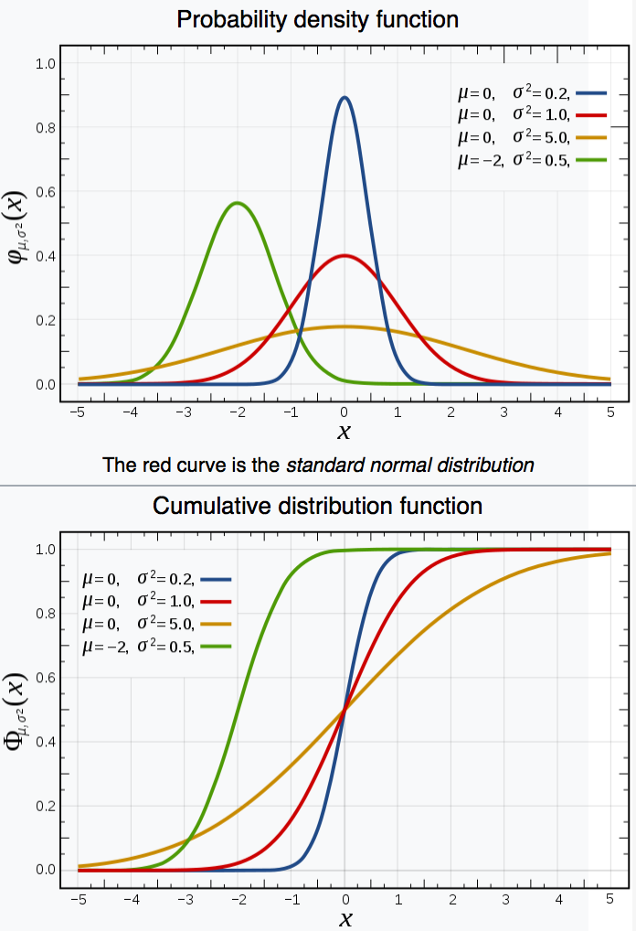
Aim : create sample (a set of values) that follows an analytic PDF
Cumulative distribution function (CDF) : Prob( X < x)
- definite integral PDF f -> CDF F
- F(b) - F(a) = P( a < X <= b ) = Integral a->b f(x) dx
- monotonically increasing function, CDF(-inf) = 0, CDF(inf) = 1
Map uniform randoms onto probabilities
- integrate PDF -> CDF (mapping PDF domain onto probability [0,1] )
- invert the CDF, so domain becomes [0,1]
- inverted_CDF(uniform random) -> sample value
Intuitively : throw randoms uniformly "vertically"
- Sigmoid CDF : low probability close to zero or 1 corresponding to tails
- greater probability in high PDF areas
- extreme case of delta-function PDF : all probability at one value
- sigmoid CDF becomes Heaviside step-function
CDF "encodes" shape of PDF in convenient form for sampling
Monte Carlo Method : Modelling Scintillator Re-emission
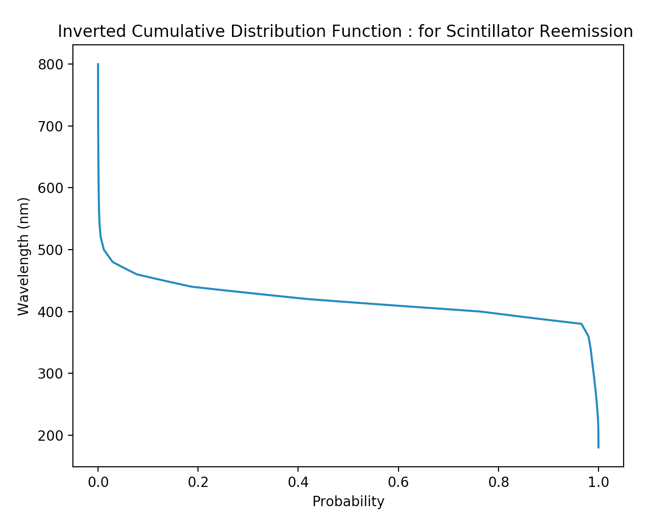
- reemission_probability(wavelength)
- fraction of light absorbed in scintillator re-emitted with different wavelength.
- generating re-emitted wavelength
- expected PDF(wavelength) -> inverted_CDF(probability)
Opticks Re-emission model
- fraction of absorbed photons "reincarnated" in same thread
- inverted_CDF(probability) -> GPU "re-emission" texture
float uniform_sample_reemit = curand_uniform(&rng);
if (uniform_sample_reemit < reemission_probability )
{
    ...
    p.wavelength = reemission_lookup(curand_uniform(&rng));    # re-emission texture lookup
    s.flag = BULK_REEMIT ;
    return CONTINUE;
}
else
{
    s.flag = BULK_ABSORB ;
    return BREAK;
}
https://bitbucket.org/simoncblyth/opticks/src/default/optixrap/cu/propagate.h
Monte Carlo Method : Modelling Scattering and Absorption
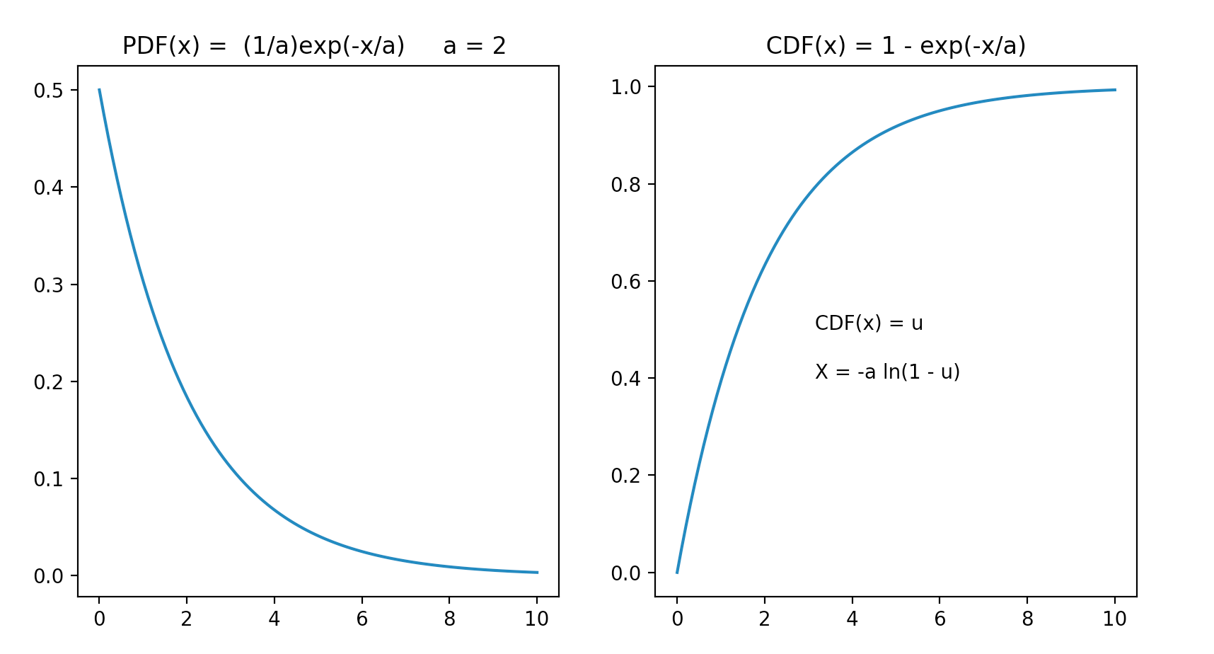
Create sample with exponential PDF, using CDF
- PDF(x) = (1/a) exp(-x/a)
- CDF(x) = 1 - exp(-x/a)
- a
- characteristic scale of process, eg decay time or scattering/absorption/attenuation length
- u
- uniform random value in [0,1] ; 1-u equivalent to u
Known analytic form of CDF, means simple sampling:
Equate CDF probability with uniform random value [0,1]
- CDF(x) = 1 - exp(-x/a) = u
- exp(-x/a) = 1 - u
- X = -a ln(1-u)
- X = -a ln(u)
- X
- stochastic distance/time obtained from characteristic scale a and uniform random u
https://www.eg.bucknell.edu/~xmeng/Course/CS6337/Note/master/node50.html
Monte Carlo Method : Accept-Reject Sampling
Simple technique providing a sample that follows a distribution. Example PDF : pdf(x) = (3/8).( 1 + x^2 )
- scatter random points (x,y) across PDF graph (piecewise for better efficiency)
- accept x for pdf(x) < y : implement in C++ with do { } while ( condition )
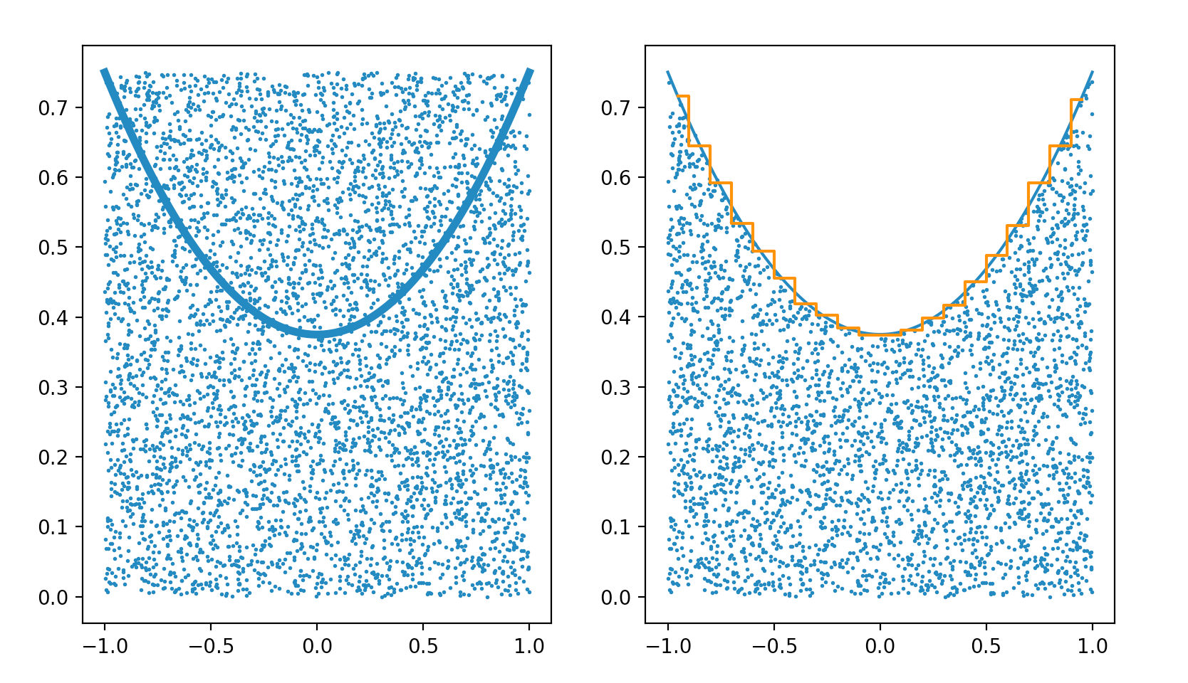
https://bitbucket.org/simoncblyth/intro_to_numpy/src/default/accept_reject_sampling.py
MC Method : Estimating Pi from circle/square count ratio : pi r^2/(2r)^2
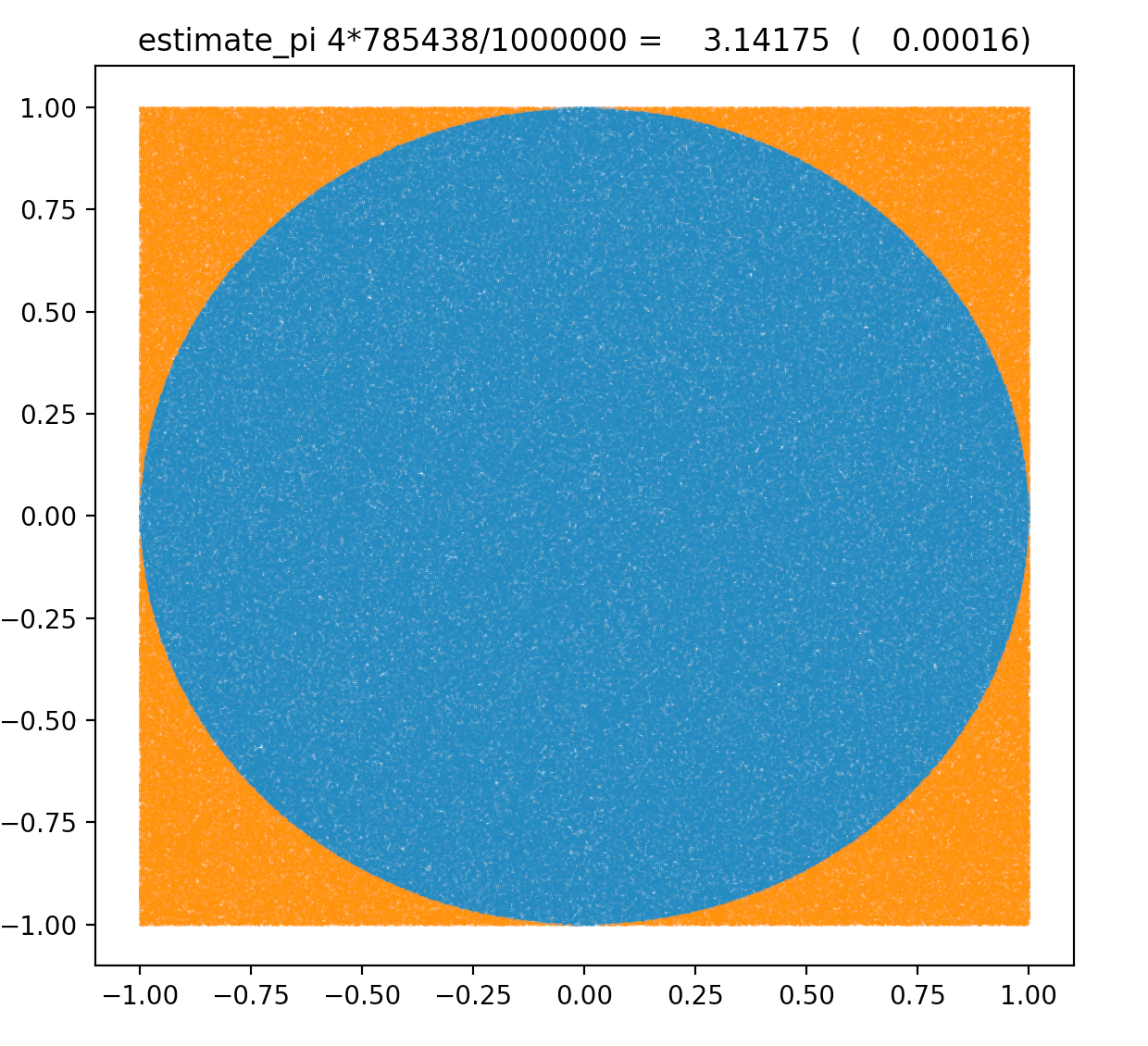
https://bitbucket.org/simoncblyth/intro_to_numpy/src/default/estimate_pi.py
Outline of Opticks : Problem, Solution, Geometry, Validation
- Optical Photon simulation problem, hybrid solution : Geant4 + Opticks
- Ray Traced Image Synthesis ≈ Optical Photon Simulation
- NVIDIA OptiX Ray Tracing Engine
- BVH : Boundary Volume Hierarchy
- BVH Pascal : software emulation
- BVH Turing : hardware "RT Cores"
- Primitives
- GPU Geometry starts from ray-primitive intersection
- Torus : much more difficult/expensive than other primitives
- CSG : Constructive Solid Geometry modelling
- Shapes defined "by construction"
- Which primitive intersect to pick ?
- Ray intersection with general CSG binary trees, on GPU
- Complete Binary Tree Serialization -> simplifies GPU side
- Evaluative CSG intersection Pseudocode : recursion emulated
- CSG Deep Tree : JUNO "fastener", balancing reduces tree height: 11 -> 4
- Geometry visualizations : Daya Bay Near Site, JUNO Central Detector
- CSG : (Cylinder - Torus) PMT neck : spurious intersects
- CSG : Alternative PMT neck designs
- Translation
- Auto-Instancing
- Opticks : translates G4 geometry to GPU, without approximation
- Opticks : Export of G4 geometry to glTF 2.0
- Opticks : translates G4 optical physics to GPU
- Validation : Opticks/G4 statistical comparison
- Simple Lights/Geometries
- 1M Rainbow S-Polarized
- Random Aligned Validation -> direct comparison
- Take Control of Geant4 Random Number Generator (RNG)
- Aligning CPU and GPU Simulations
- Direct comparison of GPU/CPU NumPy arrays
- Coincident Faces are Primary Cause of Issues : Spurious Intersects
- Summary
Ray Traced Image Synthesis ≈ Optical Photon Simulation
Geometry, light sources, optical physics ->
- pixel values at image plane
- photon parameters at detectors (eg PMTs)
Ray tracing has many applications :
- advertising, design, entertainment, games,...
- BUT : most ray tracers just render images
Ray-geometry intersection
- hw+sw continuously optimized over 30 years
- NVIDIA : "10+ Giga-ray intersections per second per GPU" (Turing GPU : hardware BVH acceleration )
- ray tracing
- cast rays thru image pixels into scene, recursively reflect/refract at intersects, combine returns into pixel values
- rasterization
- project 3D primitives onto 2D image plane, combine fragments into pixel values
NVIDIA® OptiX™ Ray Tracing Engine -- http://developer.nvidia.com/optix
Analogous to OpenGL rasterization pipeline:
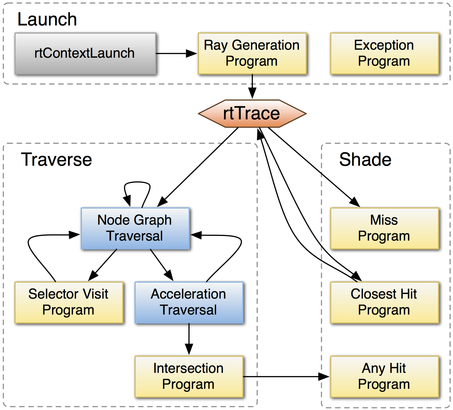
OptiX makes GPU ray tracing accessible
- accelerates ray-geometry intersections
- simple : single-ray programming model
- "...free to use within any application..."
NVIDIA expertise:
- ~linear scaling with CUDA cores across multiple GPUs
- acceleration structure creation + traversal (Blue)
- instanced sharing of geometry + acceleration structures
- compiler optimized for GPU ray tracing
- regular updates, profit from new GPU features:
- NVIDIA RTX™ with Volta, Turing GPUs
https://developer.nvidia.com/rtx
User provides (Yellow):
- ray generation
- geometry bounding box, intersects
Opticks : GPU Geometry starts from ray-primitive intersection
- 3D parametric ray : ray(x,y,z;t) = rayOrigin + t * rayDirection
- implicit equation of primitive : f(x,y,z) = 0
- -> polynomial in t , roots: t > t_min -> intersection positions + surface normals
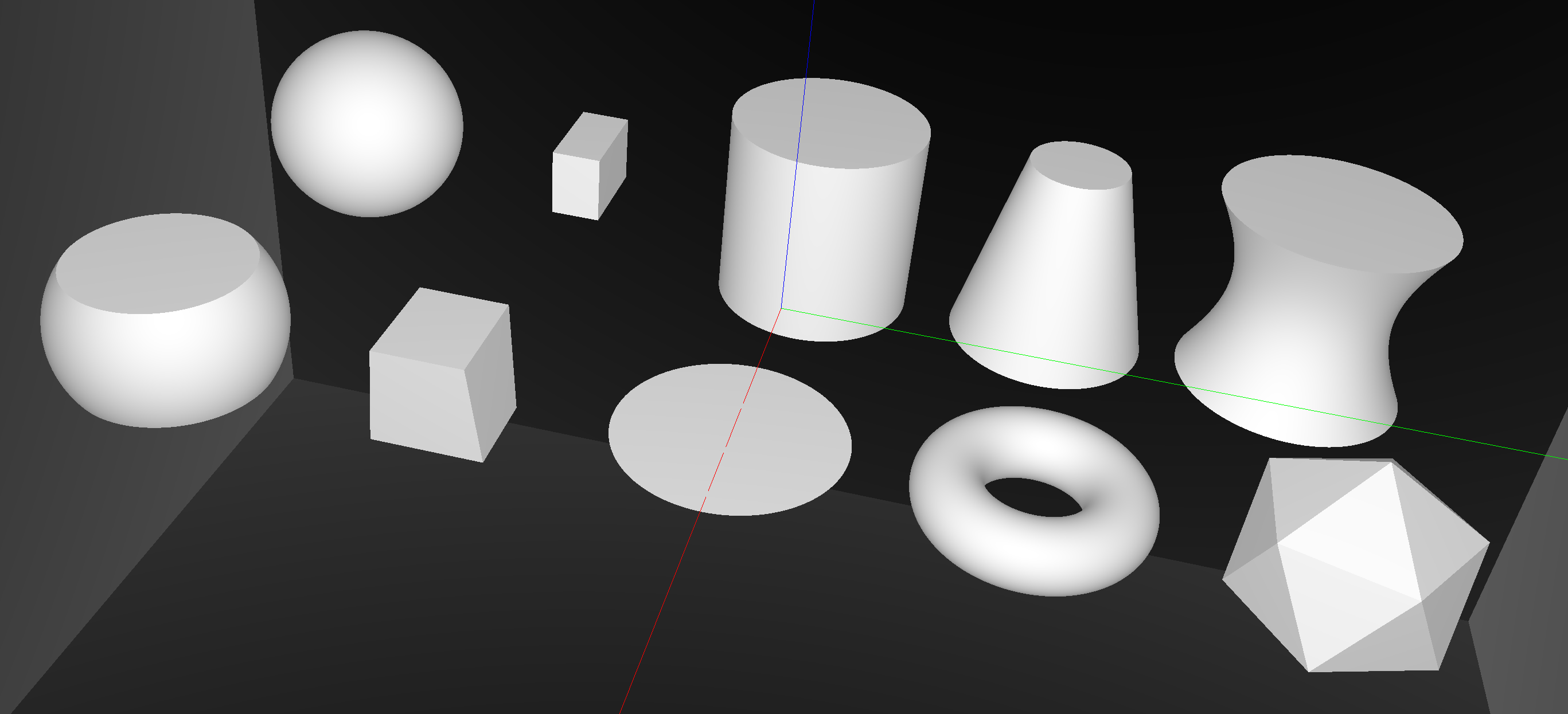
CUDA/OptiX intersection for ~10 primitives -> Exact geometry translation
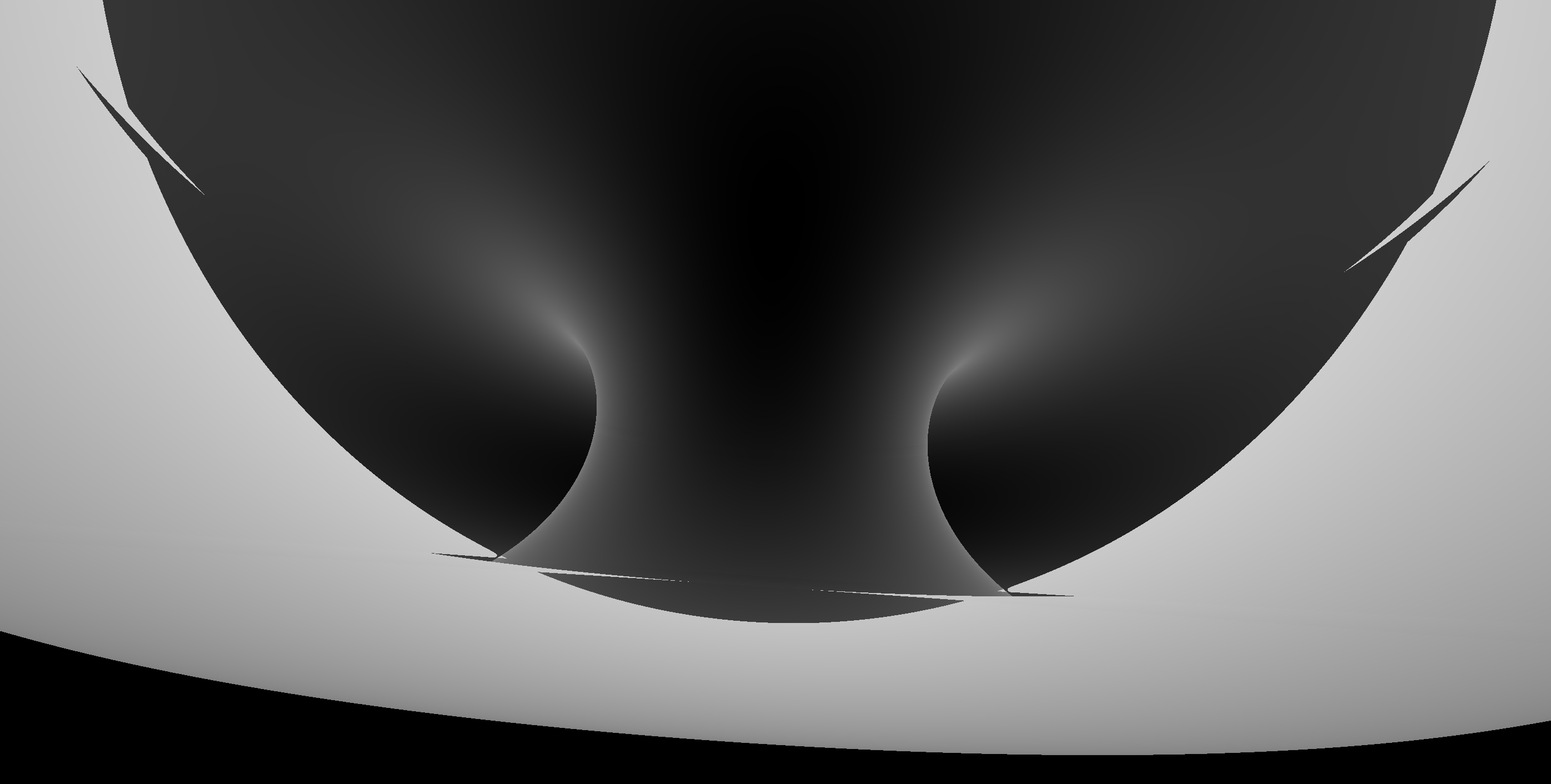
Torus : much more difficult/expensive than other primitives
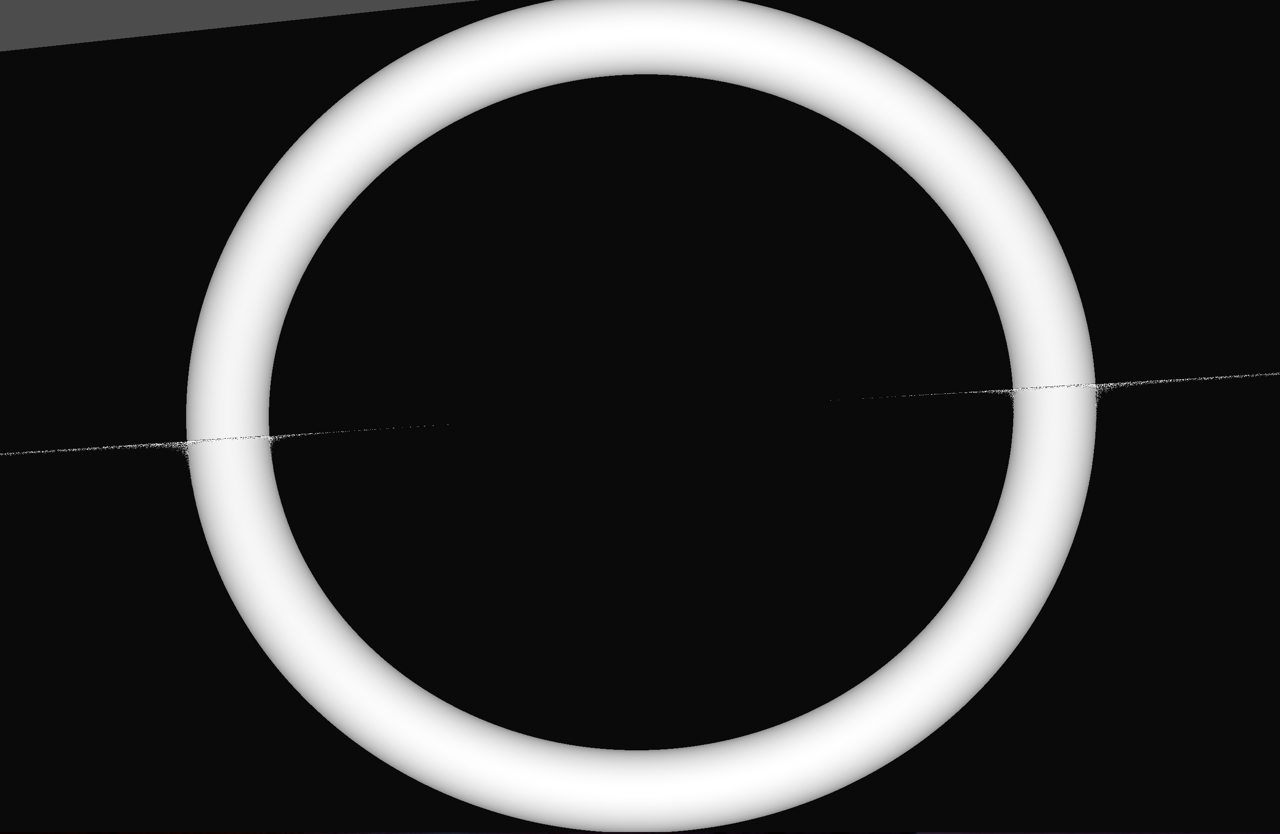
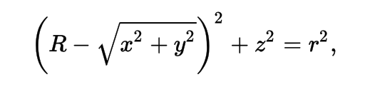
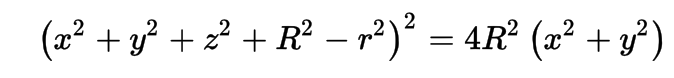
3D parametric ray : ray(x,y,z;t) = rayOrigin + t * rayDirection
- ray-torus intersection -> solve quartic polynomial in t
- A t^4 + B t^3 + C t^2 + D t + E = 0
High order equation
- very large difference between coefficients
- varying ray -> wide range of coefficients
- numerically problematic, requires double precision
- several mathematical approaches used
Best Solution : replace torus
- eg model PMT neck with hyperboloid, not cylinder-torus
Torus : different artifacts as change implementation/params/viewpoint
- Only use Torus when there is no alternative
- especially avoid CSG combinations with Torus
Constructive Solid Geometry (CSG) : Shapes defined "by construction"
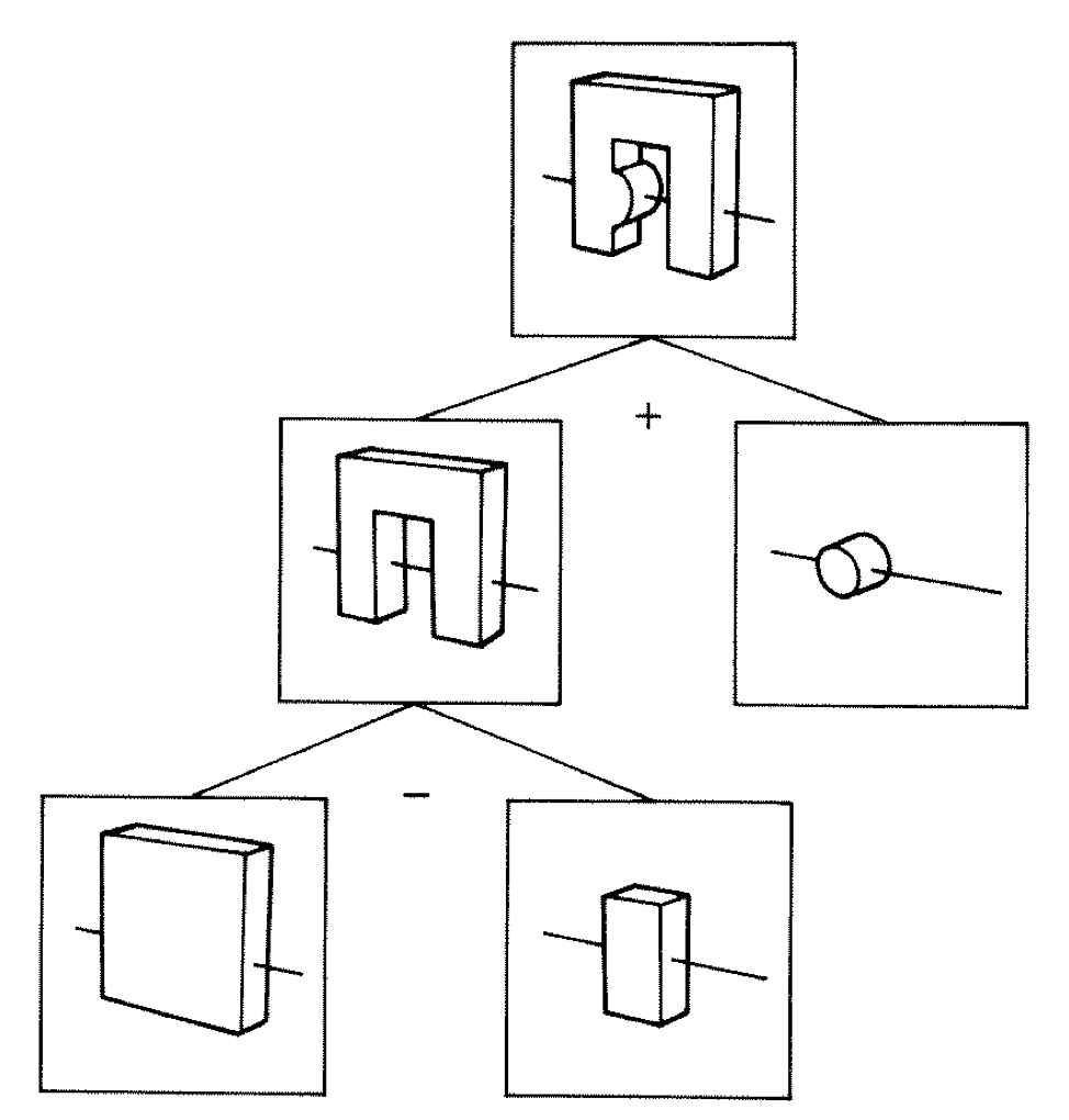
Primitives combined via binary operators
Simple by construction definition, implicit geometry.
- A, B implicit primitive solids
- A + B : union (OR)
- A * B : intersection (AND)
- A - B : difference (AND NOT)
- !B : complement (NOT) (inside <-> outside)
CSG expressions
- non-unique: A - B == A * !B
- represented by binary tree, primitives at leaves
3D Parametric Ray : ray(t) = r0 + t rDir
Ray Geometry Intersection
- primitive : find t roots of implicit eqn
- composite : pick primitive intersect, depending on CSG tree
How to pick exactly ?
CSG : Which primitive intersect to pick ?
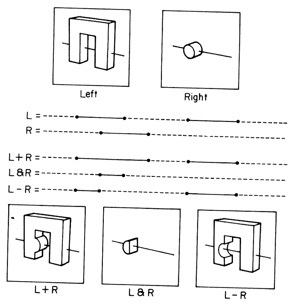
Classical Roth diagram approach
- find all ray/primitive intersects
- recursively combine inside intervals using CSG operator
- works from leaves upwards
Computational requirements:
- find all intersects, store them, order them
- recursive traverse
BUT : High performance on GPU requires:
- massive parallelism -> more the merrier
- low register usage -> keep it simple
- small stack size -> avoid recursion
Classical approach not appropriate on GPU
Ray intersection with general CSG binary trees, on GPU
dot(normal,rayDir) -> Enter/Exit
- A + B boundary not inside other
- A * B boundary inside other
Pick between pairs of nearest intersects, eg:
| UNION tA < tB | Enter B | Exit B | Miss B |
|---|---|---|---|
| Enter A | ReturnA | LoopA | ReturnA |
| Exit A | ReturnA | ReturnB | ReturnA |
| Miss A | ReturnB | ReturnB | ReturnMiss |
- Nearest hit intersect algorithm [1] avoids state
- sometimes Loop : advance t_min , re-intersect both
- classification shows if inside/outside
- Evaluative [2] implementation emulates recursion:
- recursion not allowed in OptiX intersect programs
- bit twiddle traversal of complete binary tree
- stacks of postorder slices and intersects
- Identical geometry to Geant4
- solving the same polynomials
- near perfect intersection match
- [1] Ray Tracing CSG Objects Using Single Hit Intersections, Andrew Kensler (2006)
- with corrections by author of XRT Raytracer http://xrt.wikidot.com/doc:csg
- [2] https://bitbucket.org/simoncblyth/opticks/src/tip/optixrap/cu/csg_intersect_boolean.h
- Similar to binary expression tree evaluation using postorder traverse.
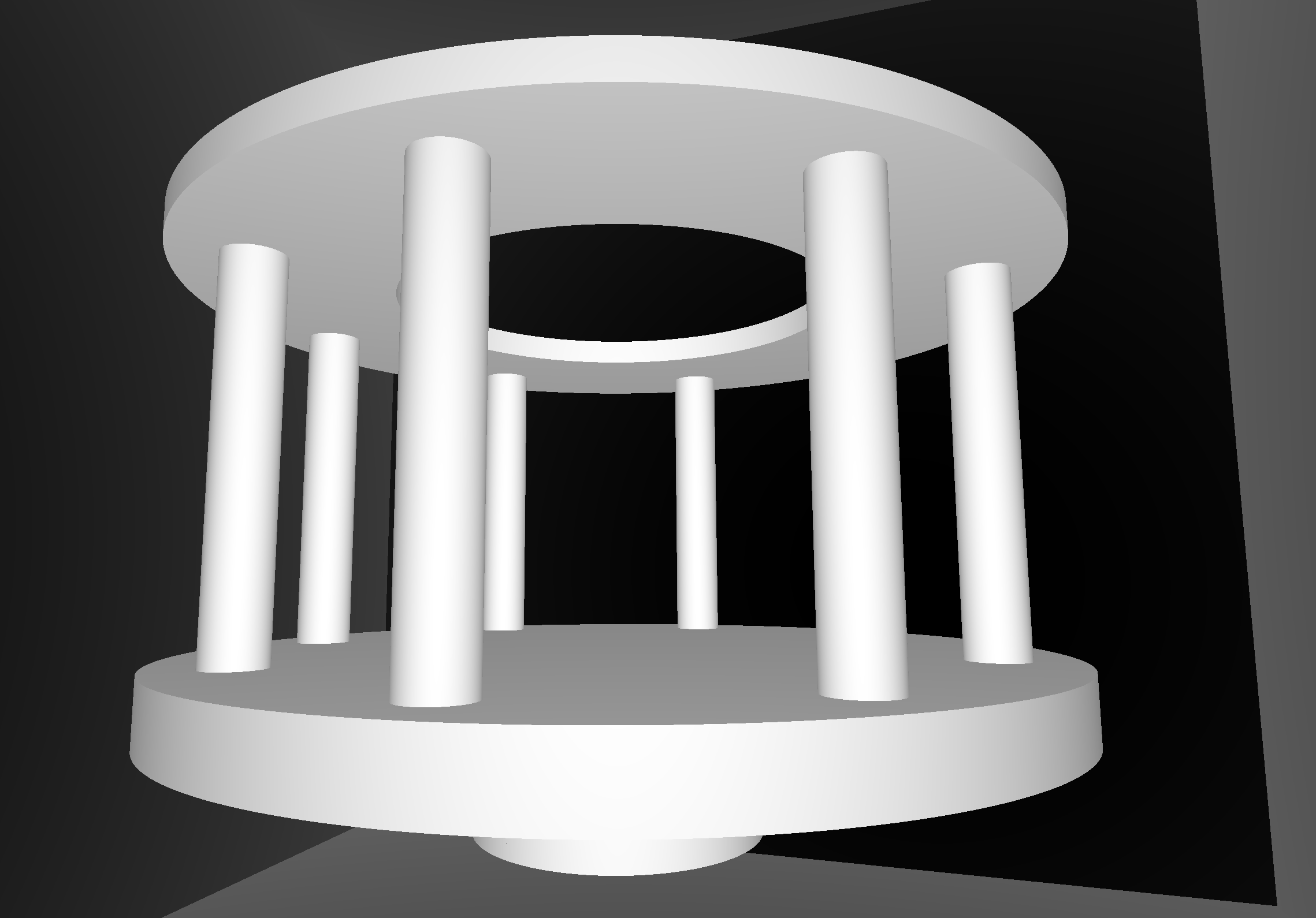
CSG Deep Tree : JUNO "fastener"
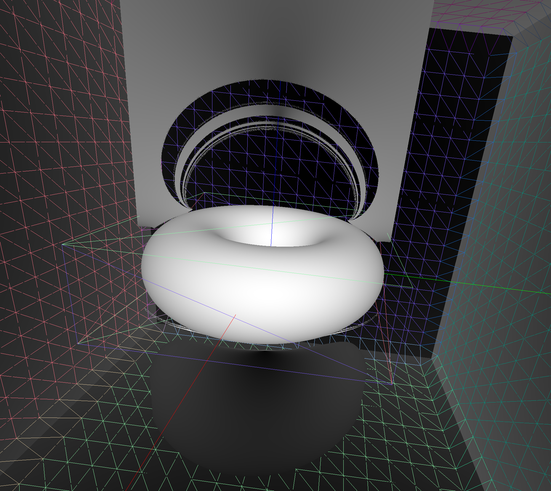
CSG : (Cylinder - Torus) PMT neck : spurious intersects
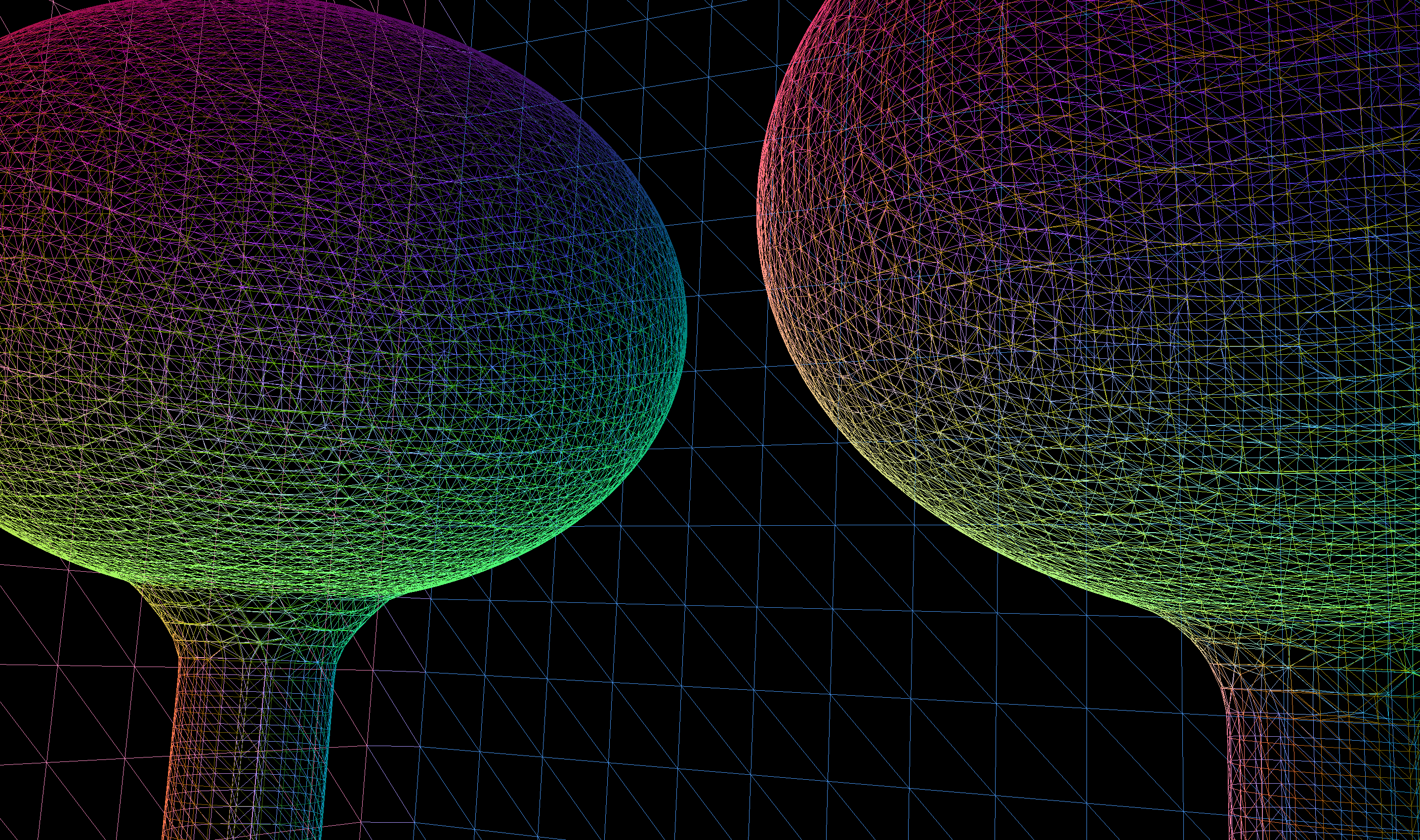
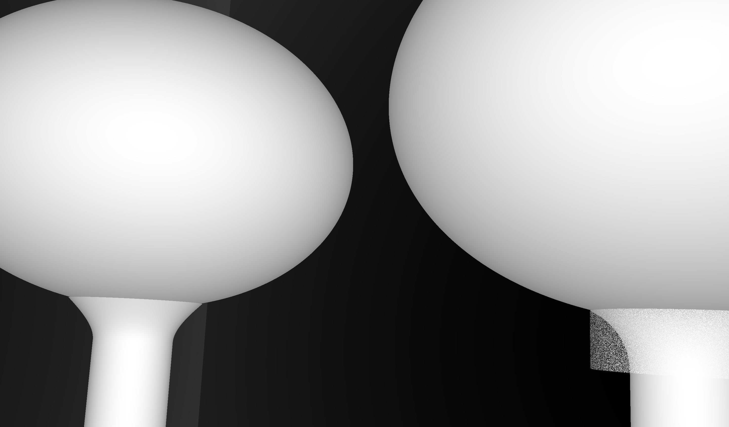
OptiX Raytrace and OpenGL rasterized wireframe comparing neck models:
- Ellipsoid + Hyperboloid + Cylinder
- Ellipsoid + (Cylinder - Torus) + Cylinder
Best Solution : use simpler neck model for physically unimportant PMT neck
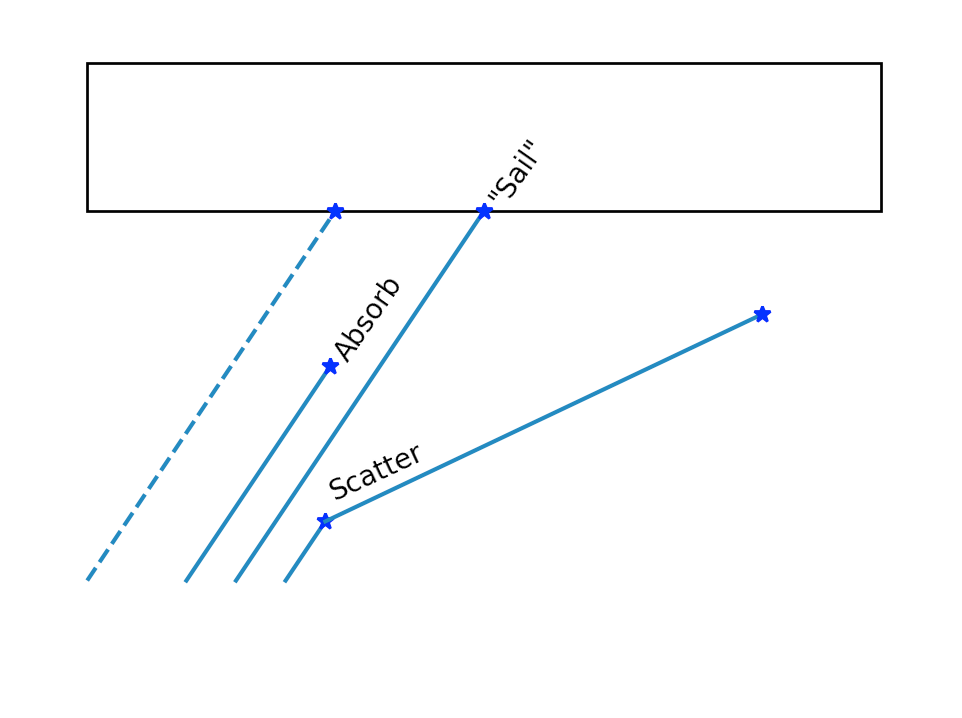
CSG : Alternative PMT neck designs
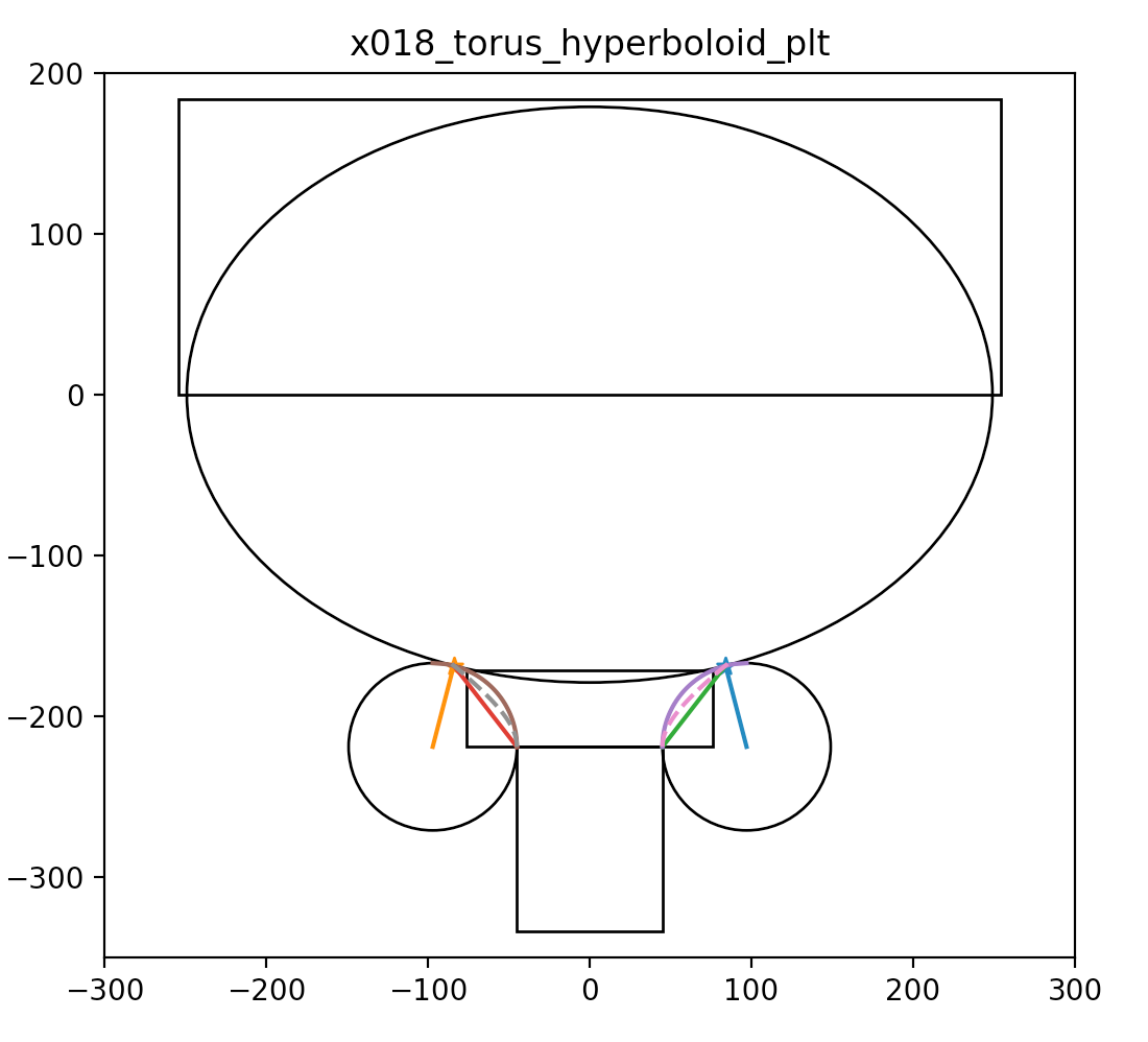
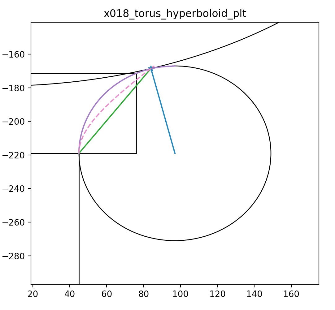
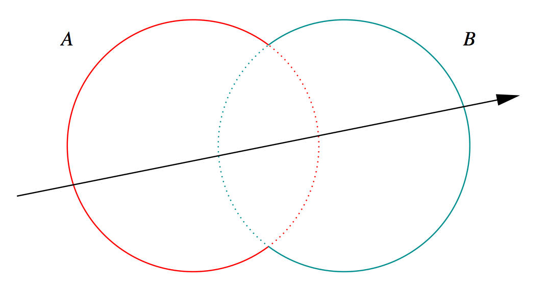
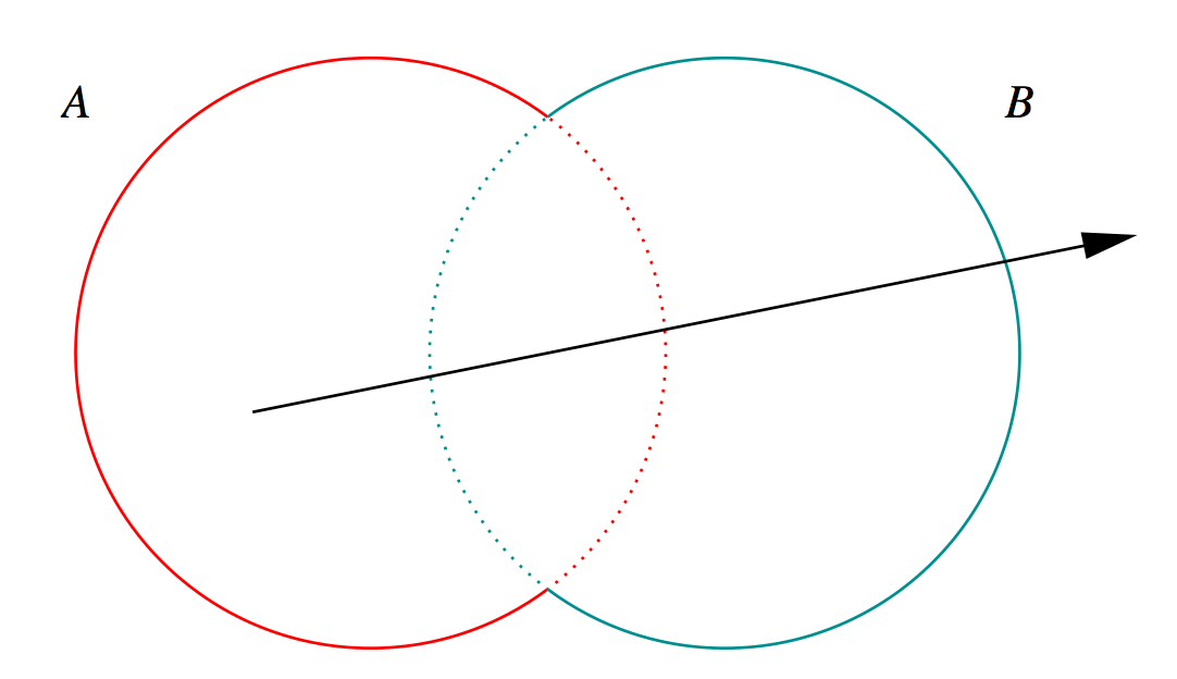
Hyperboloid and Cone defined using closest point on ellipse to center of torus circle
- Cylinder-Torus : purple line, Cone : green, simplest
- Hyperboloid : dashed magenta, works with Opticks, BUT G4Hype has no z-range flexibility
https://bitbucket.org/simoncblyth/opticks/src/tip/ana/x018_torus_hyperboloid_plt.py
Opticks Export of G4 geometry to glTF 2.0
"JPEG" of 3D

- Growing Adoption
- https://github.com/KhronosGroup/glTF https://www.khronos.org/gltf/
- <-- eg:Metal Renderer from GLTFKit
- https://github.com/warrenm/GLTFKit
- Similar to Opticks geocache
- JSON + binary buffers (eg NPY)
Opticks : translates G4 optical physics to GPU
- Seeded on GPU
- associate photons -> gensteps (via seed buffer)
- Generated on GPU, using genstep param:
- number of photons to generate
- start/end position of step
- Propagated on GPU
- Only photons hitting PMTs copied to CPU
Thrust: high level C++ access to CUDA
OptiX : single-ray programming model -> line-by-line translation
- CUDA Ports of Geant4 classes
- G4Cerenkov (only generation loop)
- G4Scintillation (only generation loop)
- G4OpAbsorption
- G4OpRayleigh
- G4OpBoundaryProcess (only a few surface types)
- Modify Cerenkov + Scintillation Processes
- collect genstep, copy to GPU for generation
- avoids copying millions of photons to GPU
- Scintillator Reemission
- fraction of bulk absorbed "reborn" within same thread
- wavelength generated by reemission texture lookup
- Opticks (OptiX/Thrust GPU interoperation)
- OptiX : upload gensteps
- Thrust : seeding, distribute genstep indices to photons
- OptiX : launch photon generation and propagation
- Thrust : pullback photons that hit PMTs
- Thrust : index photon step sequences (optional)
Validation : Compare Opticks/Geant4 with Simple Lights/Geometries
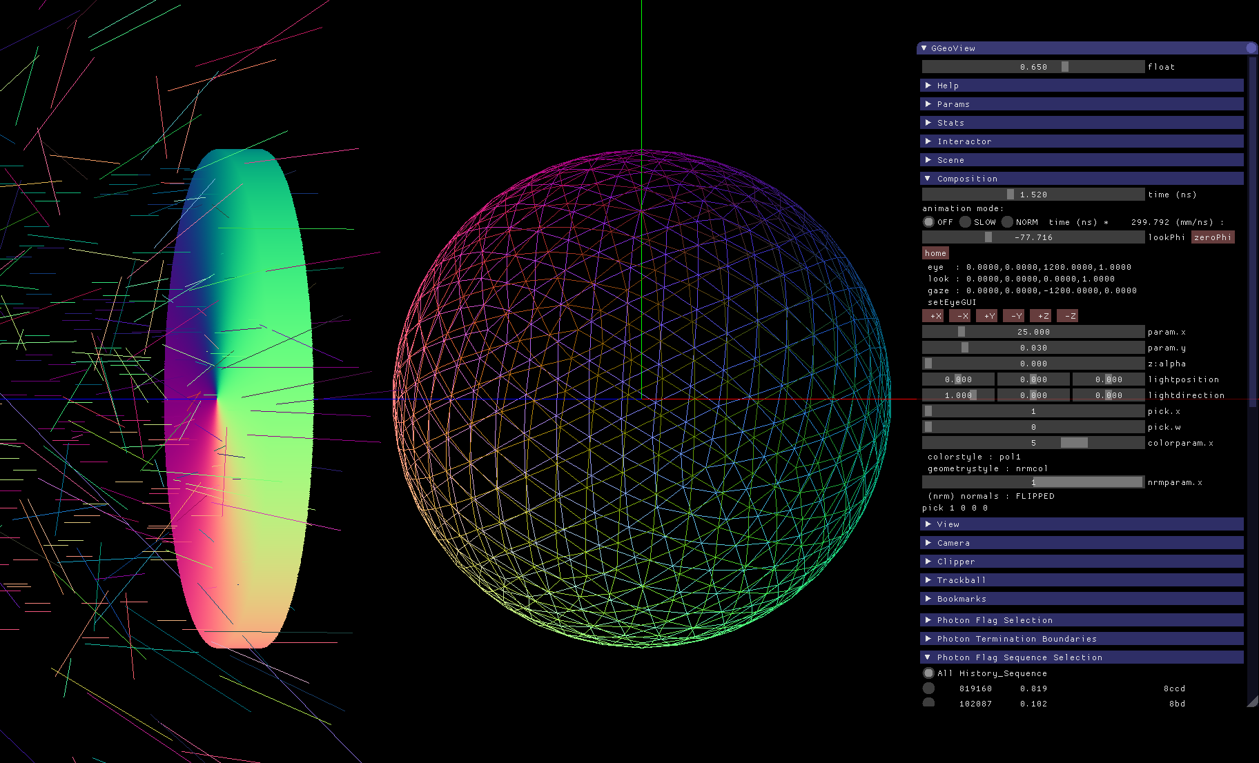
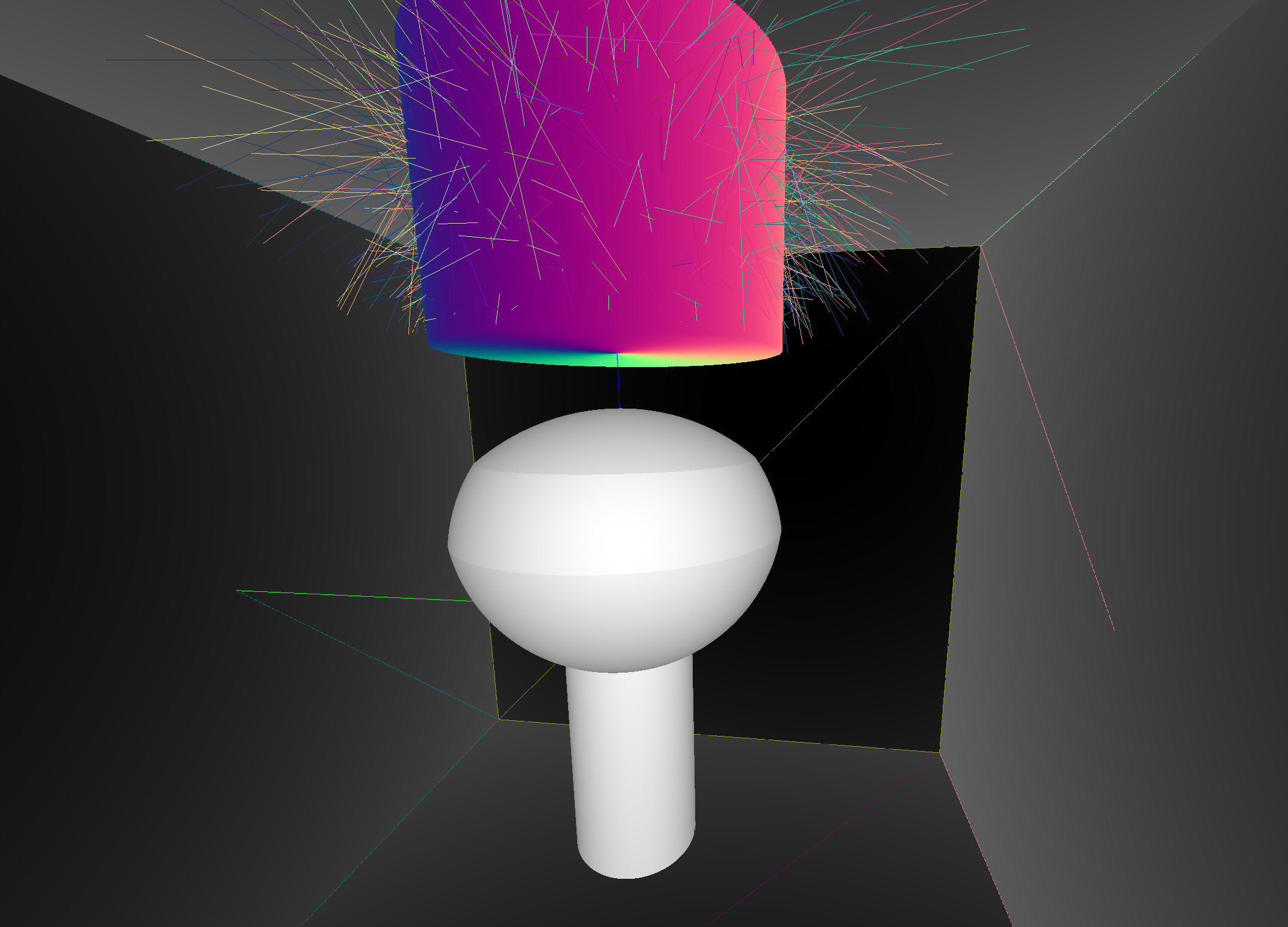
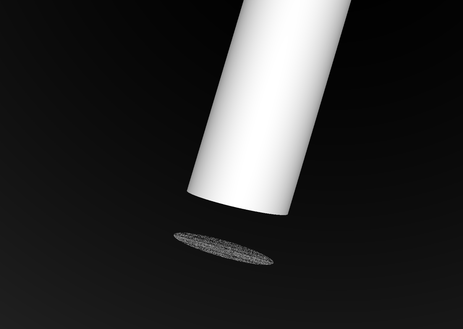
1M Photons -> Water Sphere (S-Polarized)
0.5M Photons -> Dayabay PMT
- Photon step records
- 128 bit per step : highly compressed position, time, wavelength, polarization vector, material/history codes
- Photon flag sequence
- 16x 4-bit step flags recorded in uint64 sequence, indexed using Thrust GPU sort (1M indexed ~0.040s)
- Final Photons
- Uncompressed : position, time, wavelength, direction, polarization, flags
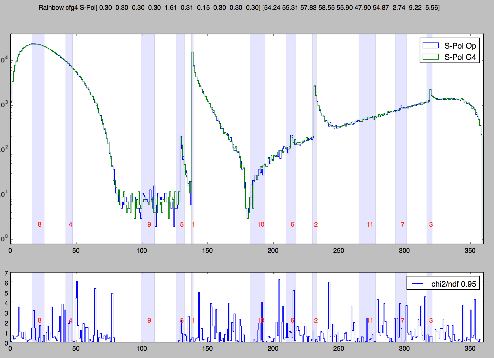
1M Rainbow S-Polarized, Comparison Opticks/Geant4
Deviation angle(degrees) of 1M parallel monochromatic photons in disc shaped beam incident on water sphere. Numbered bands are visible range expectations of first 11 rainbows. S-Polarized intersection (E field perpendicular to plane of incidence) arranged by directing polarization radially.
Coincident Faces are Primary Cause of Issues : Spurious Intersects
Coincident endcaps -> spurious intersects
Grow subtracted cone downwards, avoids coincidence : does not change composite solid
Coincidences common (alignment too tempting?). To fix:
- A-B : grow correct dimension of subtracted shape
- A+B : grow smaller interface shape into bigger, making join
- case-by-case fixes straightforward, not so easy to automate
- WIP: automated coincidence finder/fixer
Summary
Opticks enables Geant4 based simulations to benefit from effectively zero time and zero CPU memory optical photon simulation, due to massive parallelism made accessible by NVIDIA OptiX.
- Drastic speedup -> better detector understanding -> greater precision
- Performance discontinuity -> new possibilities -> imagination required
Subscribe to stay informed on Opticks: