Outline
- Context
- Photomultiplier tubes (PMTs)
- Neutrino detectors
- Current simulation approach, Geant4
- How NVIDIA OptiX can help
- Opticks : optical photon simulation with NVIDIA OptiX
- geometry migration
- porting optical physics
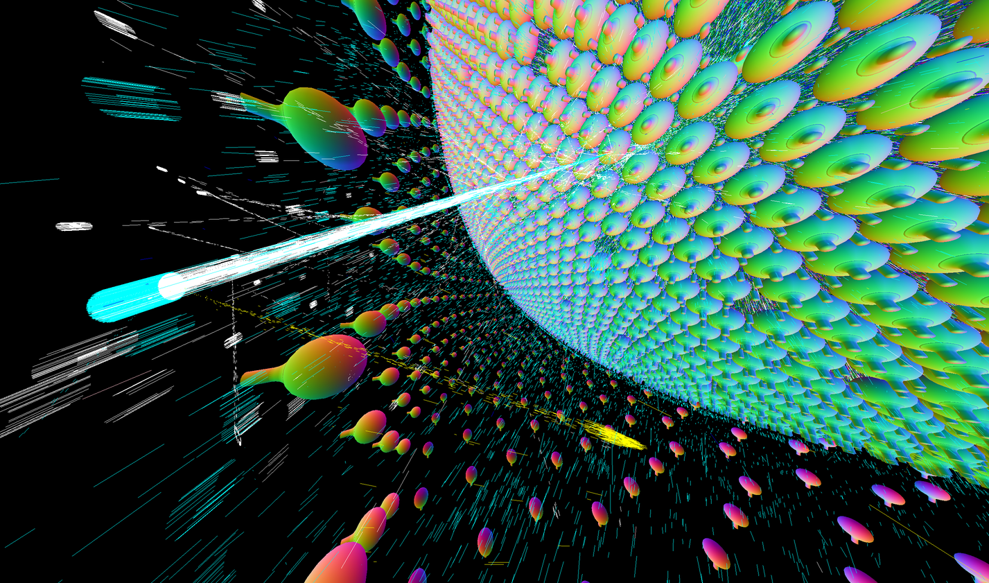
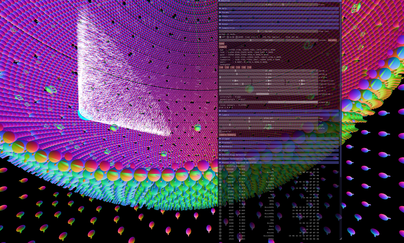
- Visualization
- Validation, performance comparisons
- Summary
- Short video
Photomultiplier Tubes (PMTs)


Photomultiplier Tube Operation
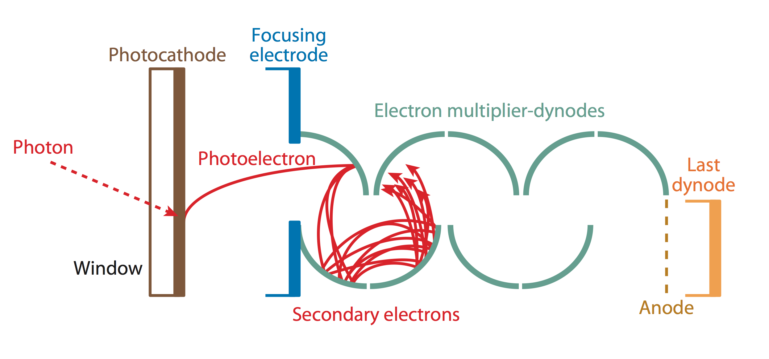
Single photoelectron amplified by ~10 dynodes to yield measurable signal
Super-Kamiokande PMTs 3
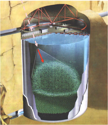
- Neutrino interaction produces charged particles travelling faster than c/n ~ 0.75c
- Cherenkov light cone seen as ring by PMTs
© Kamioka Observatory, ICRR(Institute for Cosmic Ray Research), The University of Tokyo.
Super-Kamiokande PMTs 2
© Kamioka Observatory, ICRR(Institute for Cosmic Ray Research), The University of Tokyo.
- First observation of neutrino oscillation
- upward going ~ 0.5 downward going
- -> non-zero neutrino mass
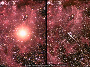
- Observed supernova 1987a burst neutrinos
- 11 neutrinos over 10s
- from nearby galaxy (~160,000 light years)
Jiangmen Underground Neutrino Observatory (JUNO)
- neutrino mass heirarchy determination
- 20 kTon liquid scintillator sphere
- 53km from 2 nuclear power plants
- energy resolution: 3% (at 1 Mev)
- PMTs: 17k 20", 17-35k 3"
- precise oscillation parameter measurement
- study neutrinos from many sources
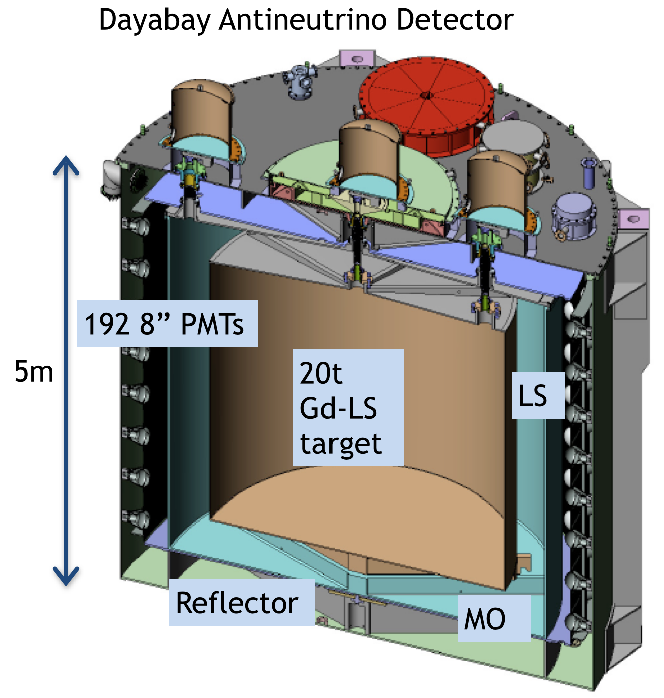
Daya Bay Far Site 2
Antineutrinos interact with proton of detector --> positron(e+) and neutron (n).
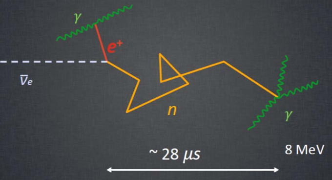
- e+ annihilates, energy deposited in scintillator re-emitted as flash of light
- delayed 2nd flash when gadolinium captures neutron and gamma energy deposited in scintillator
Distinctive double flash of light signature
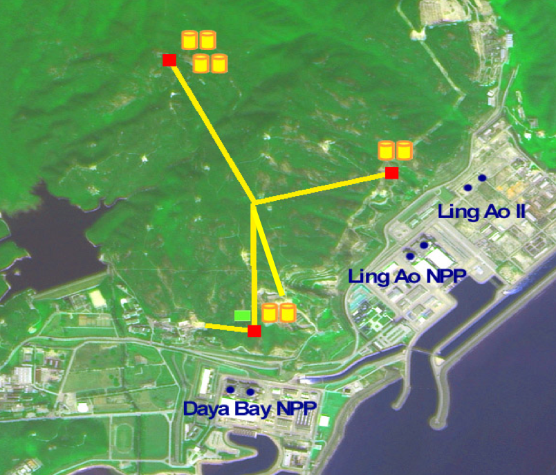
Daya Bay Far Site 3
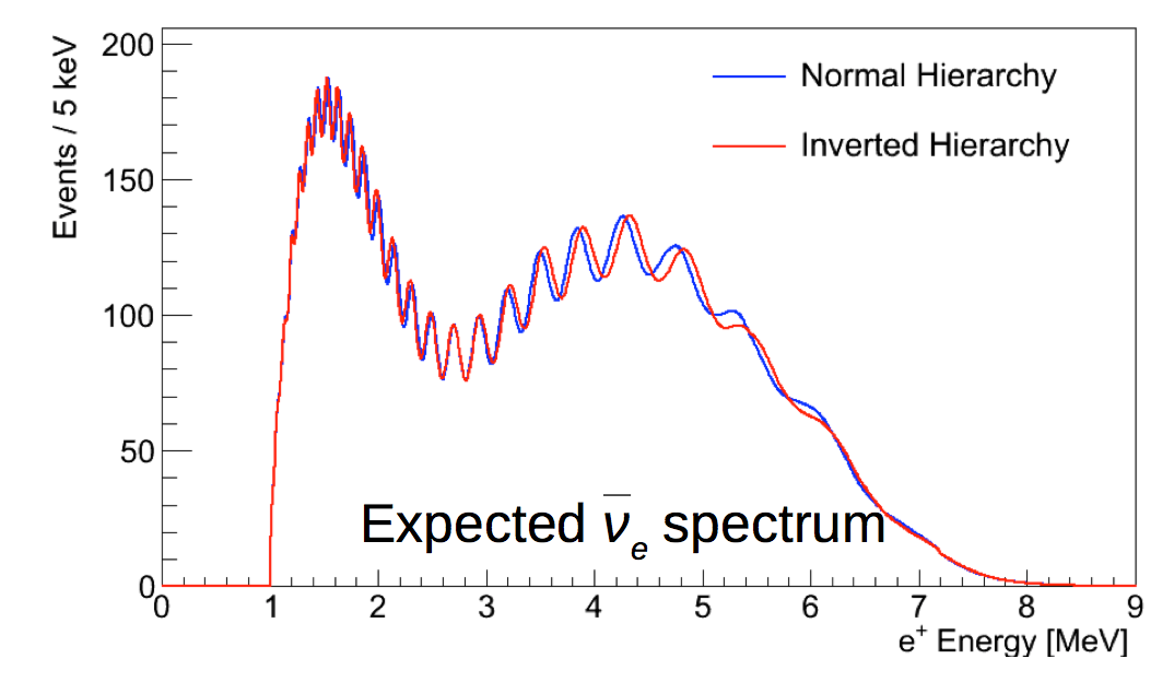
Reactor antineutrino measurements
- Most precise oscillation parameter, theta_13
- Far site baseline ~ 1.9km
- Near/Far comparison : Antineutrino Disappearance
- Most precise antineutrino spectrum
Ray Traced Realistic Image Synthesis and Optical Photon Simulation
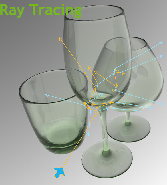
- parallel problems, just different focus
- same limit : geometry intersection
Fast ray tracing can revolutionize optical photon simulation
NVIDIA OptiX Ray Tracing Engine:
- state-of-the-art GPU accelerated intersection
- regular releases: improvements, new GPU tuning
- shared C++/CUDA context eases development
- NVIDIA expertise on efficient GPU/multi-GPU usage
- ~linear scaling with cores across multiple GPUs
NVIDIA OptiX makes massively parallel intersection accessible
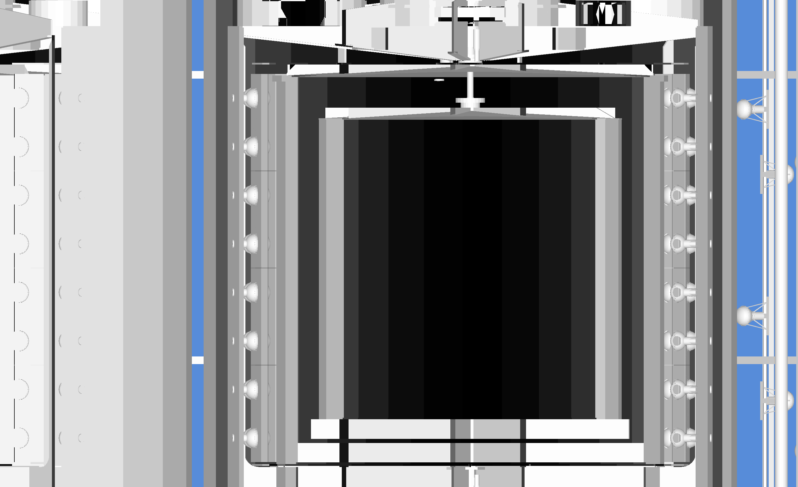
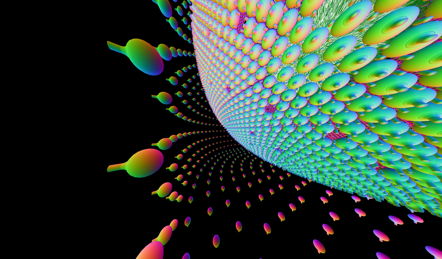
Geometry Modelling : Tesselated vs Analytic Photomultiplier Tubes
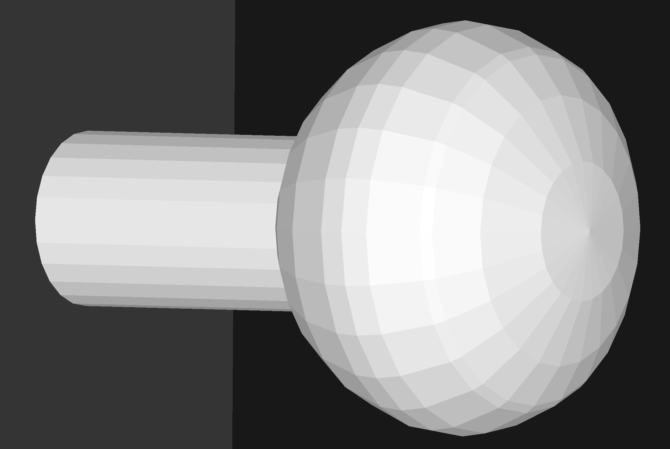
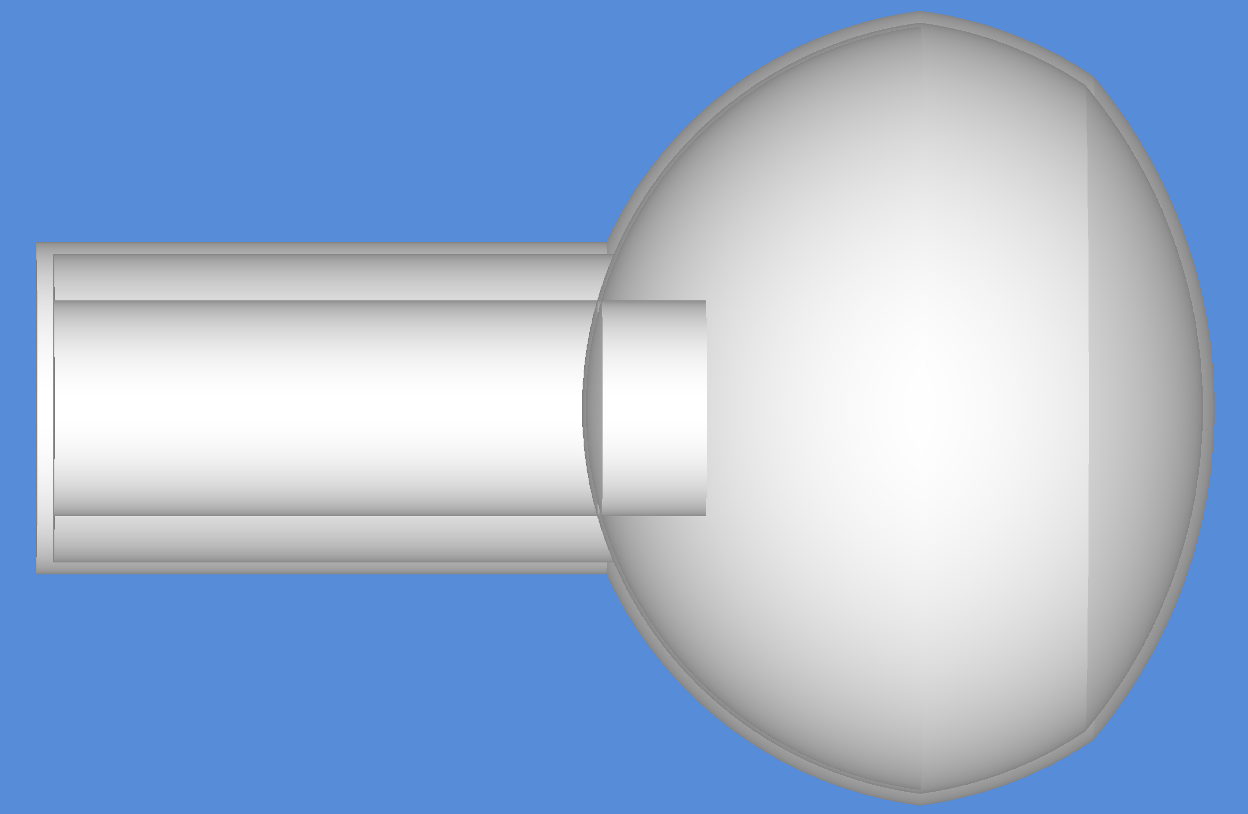
Analytic : more realistic, faster, less memory, much more effort
For Dayabay PMT:
- partition CSG solids into 12 single primitive parts (instead of 2928 triangles)
- splitting at geometrical intersections avoids implementing general CSG boolean handling
- geometry provided to OptiX in form of ray intersection code
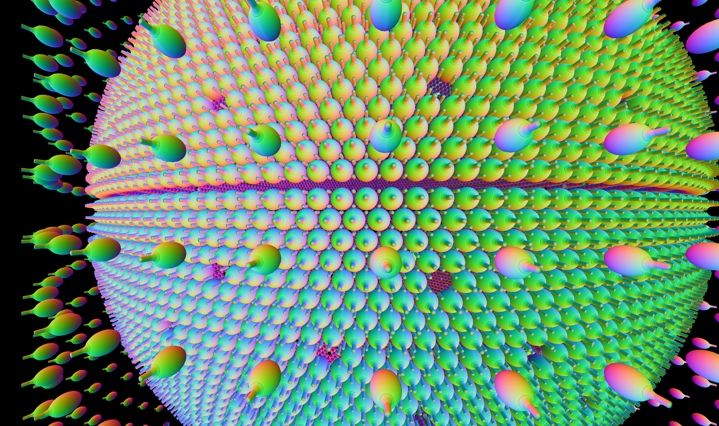
Tesselated Photomultiplier : unrealistic disco ball effect
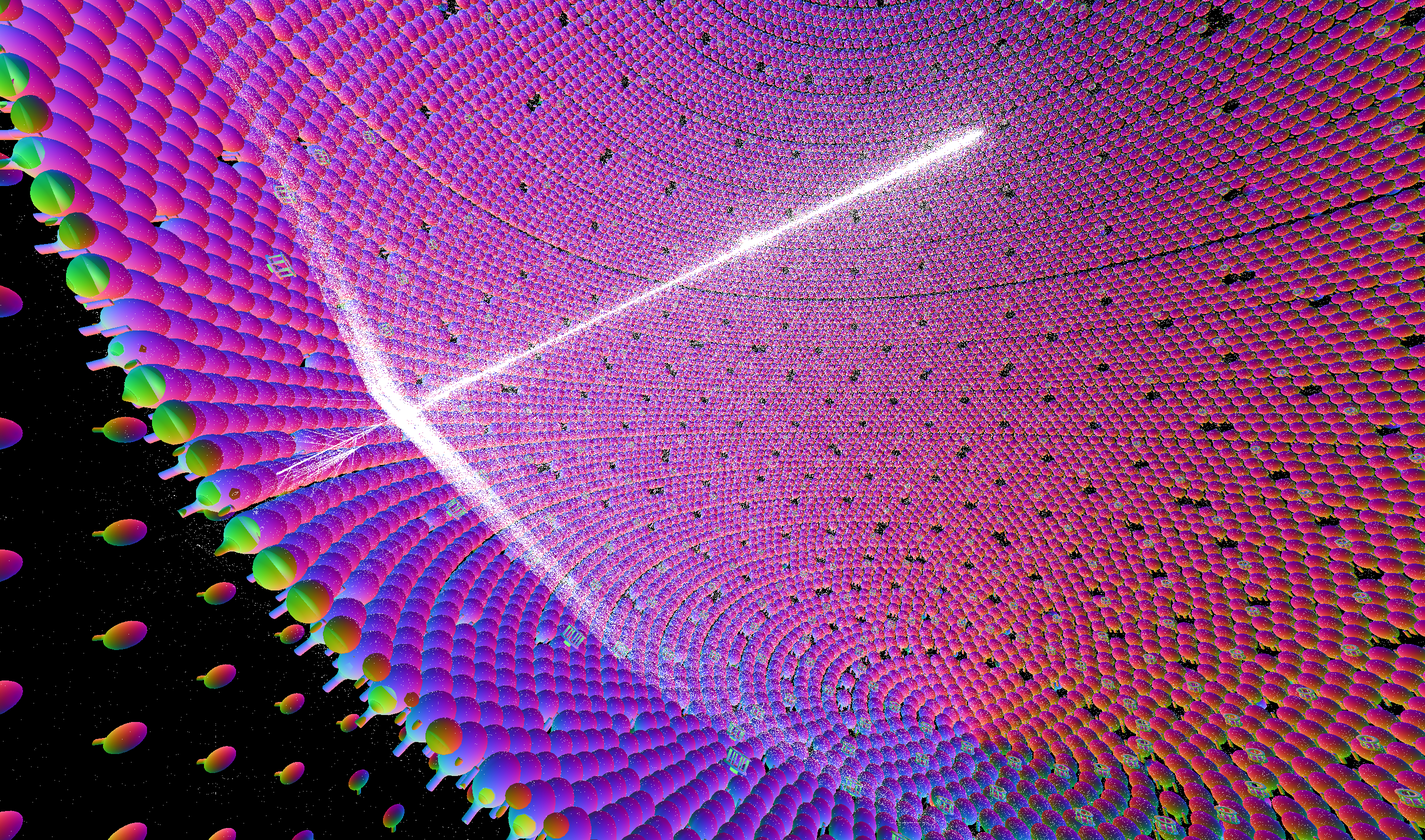
Analytic PMTs together with triangulated geometry
Starting from convenient tesselated geometry, implement analytic geometry for critical parts in primary optical path, to allow very close Geant4/Opticks match.
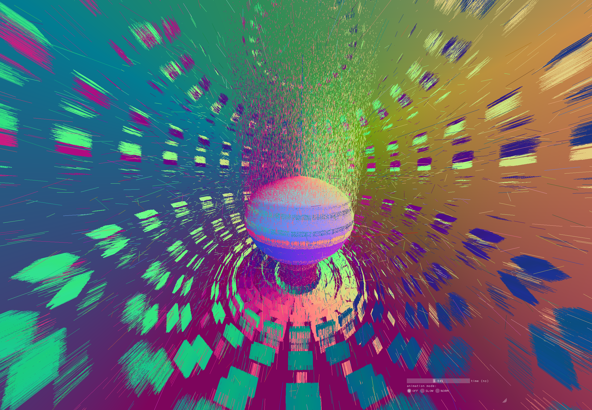
Compare Opticks/Geant4 Simulations with Simple Lights/Geometries
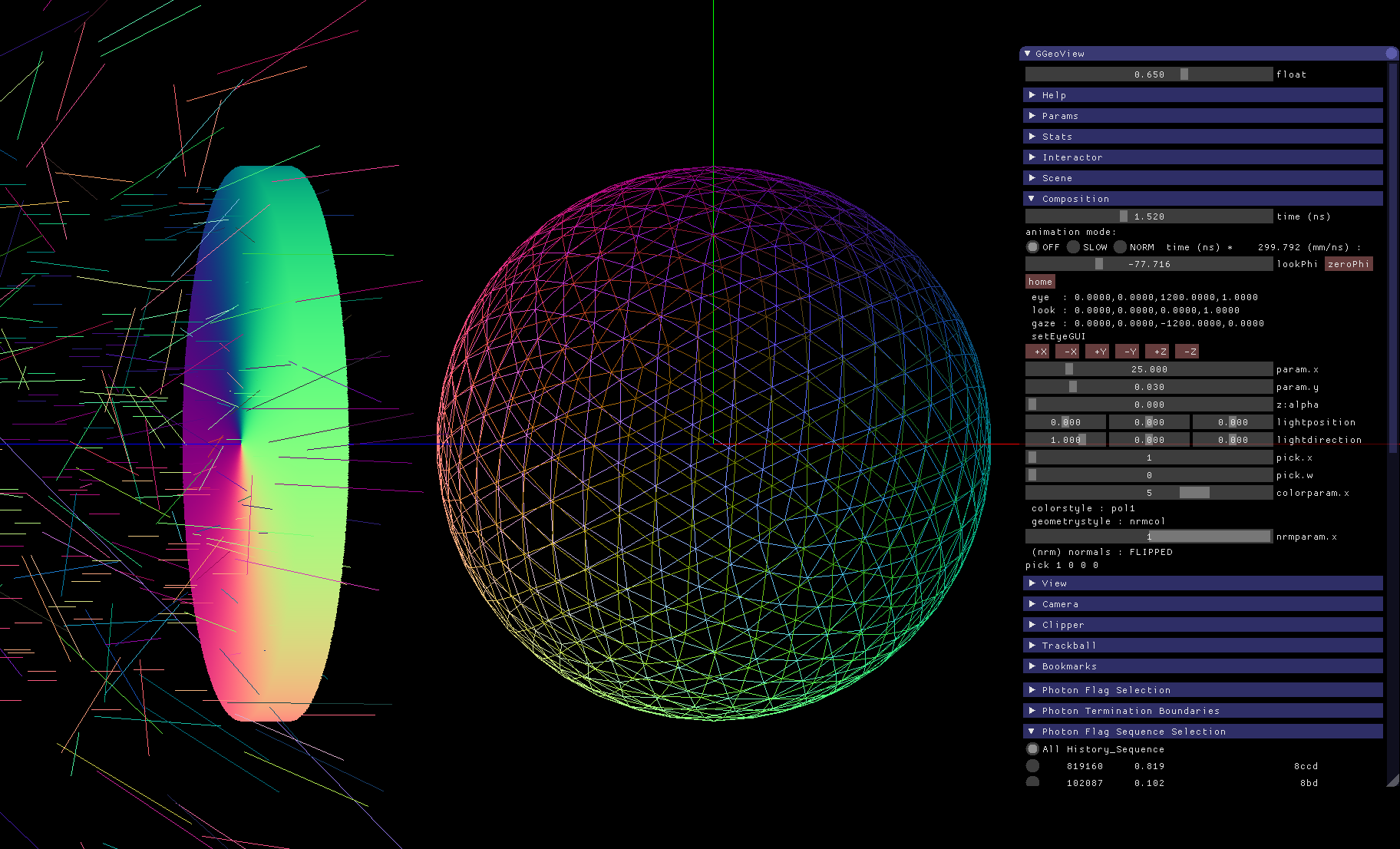
1M Photons -> Water Sphere (S-Polarized)
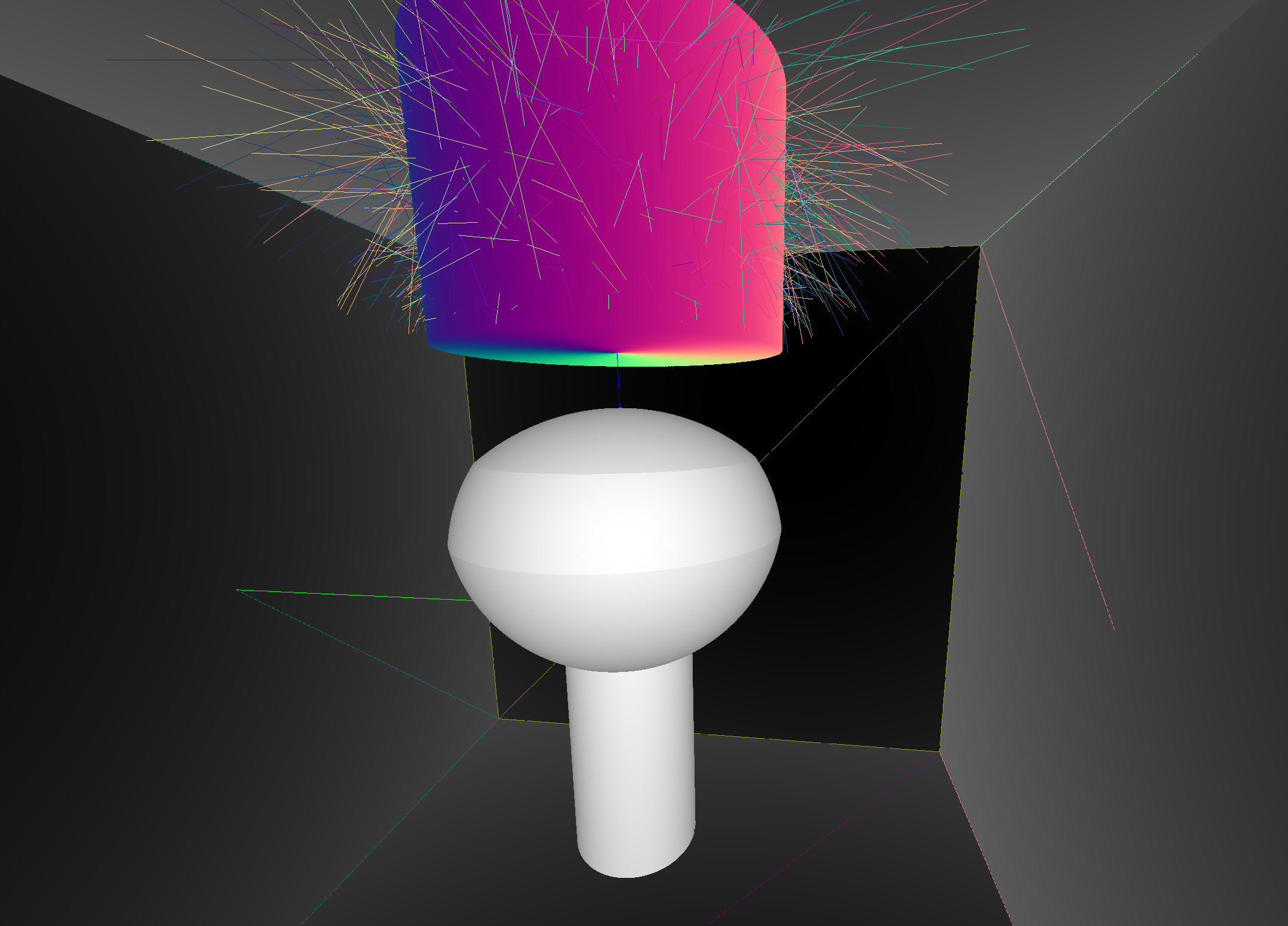
0.5M Photons -> Dayabay PMT
- record steps of all photons : position, time, wavelength, polarization vector, material/history codes
- 128 bit per step (2*short4) : snorm/uchar compressed using known domains
- water sphere : yields multiple rainbows depending on reflections
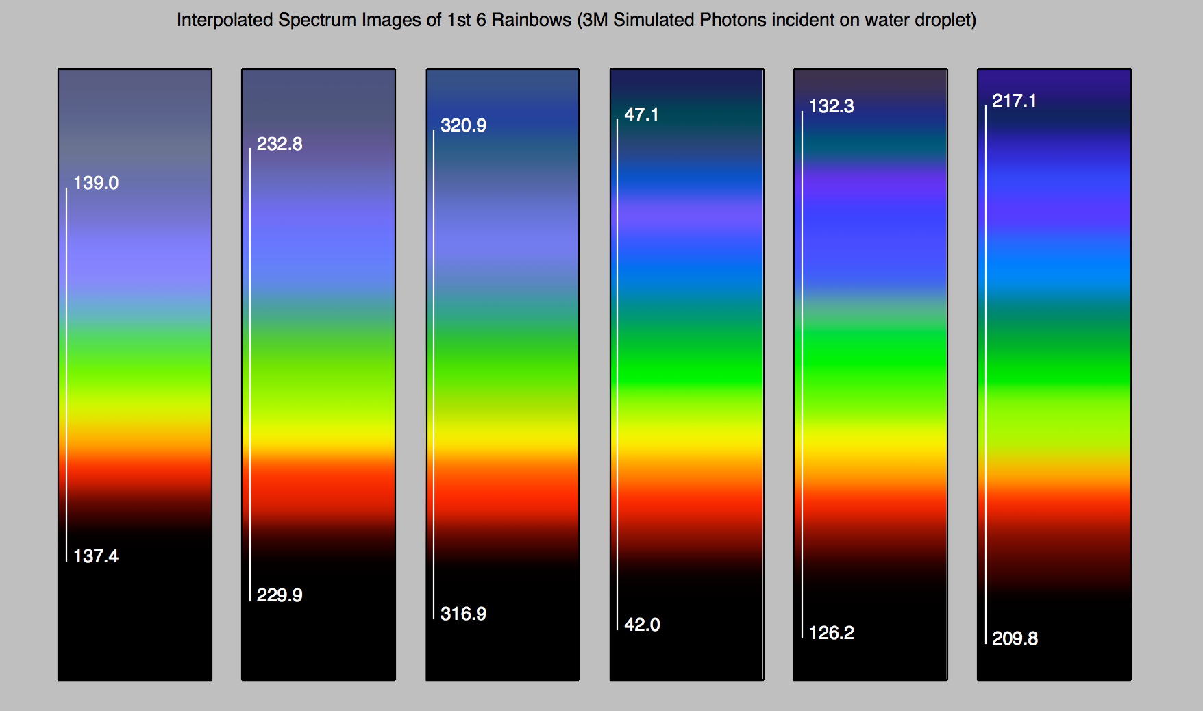
Rainbow Spectrum for 1st six bows
Spectra obtained by selecting photons by internal reflection counts. Colors obtained from spectra of each bin using CIEXYZ weighting functions converted into sRGB/D65 colorspace. Exposures by normalizing to bin with maximum luminance (CIE-Y) of each bow. White lines indicate geometric optics prediction of deviation angle ranges of the visible range 380-780nm. 180-360 degrees signifies exit on same side of droplet as incidence.
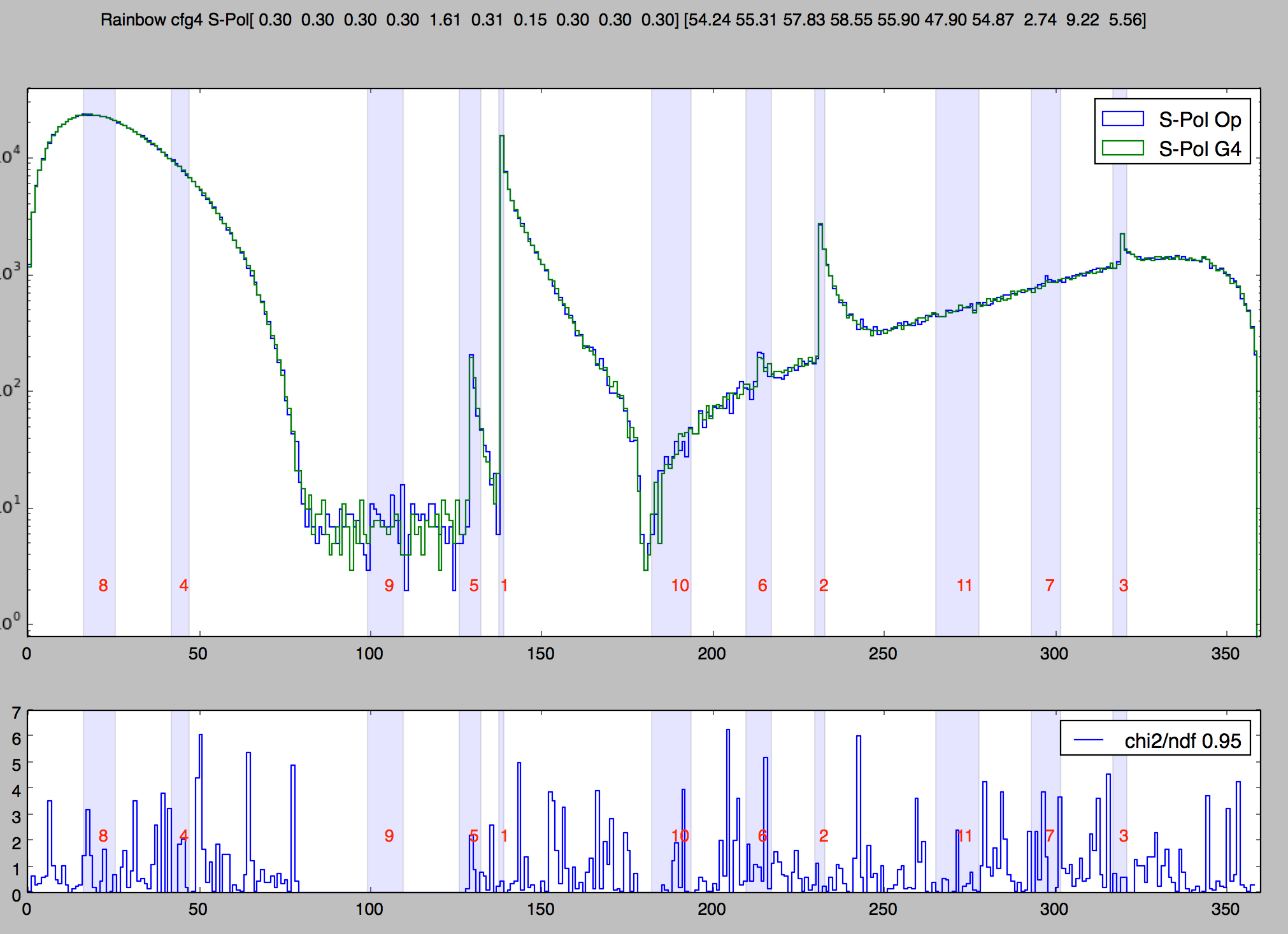
1M Rainbow S-Polarized, Comparison Opticks/Geant4
Deviation angle(degrees) of 1M parallel monochromatic photons in disc shaped beam incident on water sphere. Numbered bands are visible range expectations of first 11 rainbows. S-Polarized intersection (E field perpendicular to plane of incidence) arranged by directing polarization radially.
PMT Opticks/Geant4 step distribution comparison TO BT [SD]
Good agreement reached, after several fixes: geometry, total internal reflection, group velocity
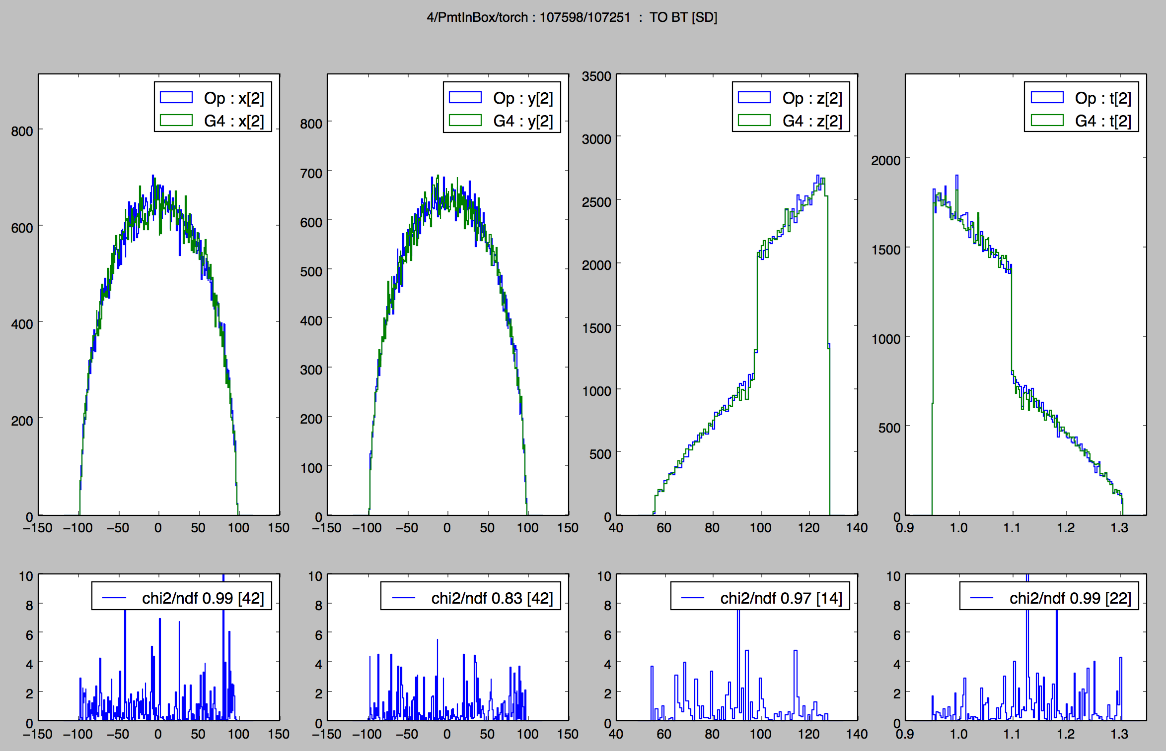
position(xyz), time(t)
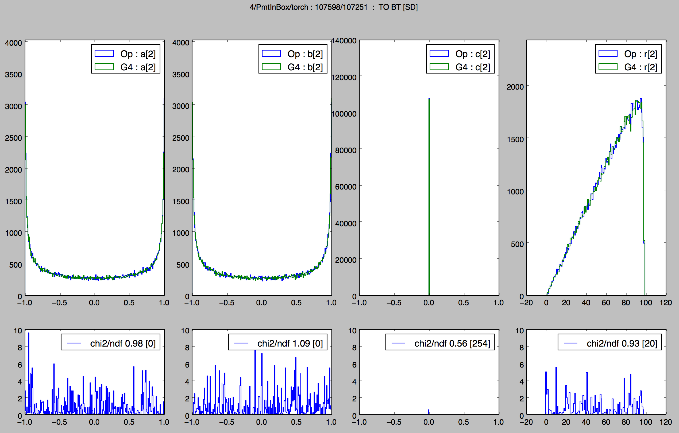
polarization(abc), radius(r)
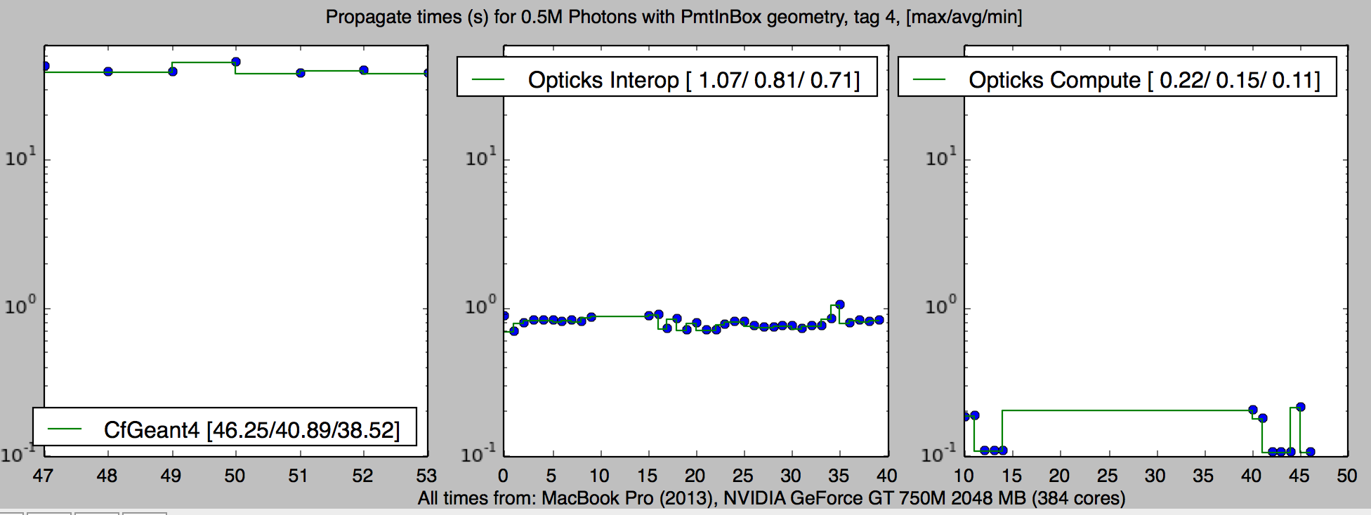
Photon Propagation Times Geant4 cf Opticks
| Test | Geant4 10.2 | Opticks Interop | Opticks Compute |
|---|---|---|---|
| Rainbow 1M(S) | 56 s | 1.62 s | 0.28 s |
| Rainbow 1M(P) | 58 s | 1.71 s | 0.25 s |
| PmtInBox 0.5M | 41 s | 0.81 s | 0.15 s |
- Opticks > 200X Geant4 with only 384 core mobile GPU[1] (multi-GPU workstation up to 20x more cores)
- photon propagation time will become effectively zero
- Interop uses OpenGL buffers allowing visualization, Compute uses OptiX buffers
- Interop/Compute : perfectly identical results, monitored by digest
[1] MacBook Pro (2013), NVIDIA GeForce GT 750M, 2048 MB, 384 cores
Summary
Opticks enables particle physics to benefit from optical photon simulation taking effectively zero time and zero CPU memory, thanks to massive parallelism made accessible by NVIDIA OptiX.
- The more photons the bigger the overall speedup (99% -> 100x)
- Drastic speedup -> better detector understanding -> greater precision
- Large PMT based neutrino experiments, such as JUNO, can benefit the most